Lower Bounds and Limitations

A lower bound says that every algorithm solving a specified problem must use at least a certain amount of a specified resource. Its force comes from the words every algorithm, together with the problem’s assumptions. A query lower bound can rule out an entire class of black-box strategies while saying little about a structured input whose description reveals a shortcut.

This page explains how to interpret such bounds when inputs must be loaded, states measured, and circuits executed with noise. The central questions are what the algorithm receives, what it must return, which inputs it must handle, and what is counted. Changing one of these can change the problem.

Helpful background. Query complexity defines oracle calls and their lower-bound methods; classical information explains input representations, output tasks and statistical error.

Lower bounds, worst cases and reductions

An algorithmic upper bound supplies a successful procedure. A lower bound must exclude every procedure in the stated model, including ones that have not yet been invented. “The fastest known method takes exponential time” therefore does not establish an exponential lower bound.

The order of the quantifiers

For an input family $D_n$, a typical worst-case statement is: every algorithm that succeeds on all allowed inputs has some input on which its cost is large. Symbolically,

$$\begin{aligned} &\forall A\text{ correct on }D_n,\\ &\qquad \max_{x\in D_n} C_A(x)\ge L(n). \end{aligned}$$

The success requirement includes the stated error probability. The maximizing input may depend on $A$. This is different from saying that one fixed input is hard for every algorithm. In a query model, a procedure specialized to a known input could simply have its answer hardwired. It would not solve the unknown-input family.

Nor does a worst-case bound describe typical inputs. Average-case statements need a specified distribution. A promise can remove the difficult instances: searching an unordered list and searching a sorted list are different tasks, even when both lists contain the same number of entries.

The size variable also matters. Dimension $d=2^n$, sparsity $s$, condition number $\kappa$, simulation time, accuracy $\epsilon$ and failure probability $\delta$ cannot all be hidden inside “problem size.” Polynomial dependence on $d$ is exponential dependence on $n$.

Which resource is bounded?

Resource	What is counted	Additional information needed for a broader conclusion
Oracle queries	Calls to a specified input operation	How the operation is implemented
State copies	Preparations consumed by an estimation task	Allowed measurements and output accuracy
Logical gates	Operations from a chosen gate library	Parallelism, connectivity and scheduling
Circuit depth	Sequential layers in a schedule	Gate durations and classical delays
Physical time	Duration under a device model	Preparation, repetitions and verification

Suppose a theorem requires $Q\ge Q_*$ queries, and one available compiler uses at most $C$ gates per call. It does not follow that $G\ge Q_*C$. An expensive construction is an upper bound on one implementation, not a lower bound on all implementations. Successive calls may even cancel: a reversible bit oracle satisfies $O_f^2=I$. An implementation can omit that pair entirely.

Lower bounds transfer through reductions in a particular direction. If solving $B$ would solve a known hard problem $A$, then a sufficiently cheap solver for $B$ is excluded. A construction that uses $A$ to solve $B$ instead supplies an upper-bound method. The reduction must preserve the promise, success requirement and counted resource.

No-fast-forwarding and structured Hamiltonians

Set $\hbar=1$ and consider sparse Hamiltonians accessed through oracles returning the locations and values of nonzero entries. Two common dimensionless evolution scales are

$$\sigma=\lVert H\rVert |t|, \qquad \tau=s\lVert H\rVert_{\max}|t|.$$

The first uses the operator norm; the second uses sparsity and the largest entry magnitude. They need not be equal.

What the black-box obstruction says

Berry, Ahokas, Cleve and Sanders construct a two-sparse family indexed by an unknown $N$-bit string. At time $t=\pi$, the evolution transfers an initial basis state to a final basis state whose extra bit is the string’s parity. For this family $\lVert H\rVert=N/2$, hence $\sigma=\pi N/2$. An algorithm simulating every member to trace-distance error at most $1/4$ needs at least $N/4=\sigma/(2\pi)$ Hamiltonian queries in the worst case Berry et al. (2007).

The reasoning is a reduction: simulation would compute the unknown parity, and each Hamiltonian query can be implemented using at most two bit queries. The parity lower bound then constrains the simulator. The algorithm must handle the family through its oracles; the claim is not that a single fully specified matrix defeats every specialized circuit.

Later sparse-oracle results give a linear-in-$\tau$ obstruction and a separate precision obstruction of order $\log(1/\epsilon)/\log\log(1/\epsilon)$ in their respective regimes Berry, Childs and Kothari (2015). Two separate lower bounds imply their maximum, not their product. See Hamiltonian simulation algorithms for the precise models and joint parameter dependence.

Why some systems can be fast-forwarded

If $H=V^\dagger D V$ and both $V$ and the diagonal phases can be implemented efficiently, then

$$e^{-iHt}=V^\dagger e^{-iDt}V.$$

Large $t$ need not require repeating a short-time circuit $t$ times. But finding $V$, computing the phases to sufficient accuracy, and specifying $t$ are real parts of this method. For example, an eigenvalue error $|\Delta E|$ produces a phase error bounded by $|t\Delta E|$. Long-time evolution can therefore require finer coefficient precision.

Explicit sums of polynomially many commuting constant-locality terms offer another route: their exponentials factor exactly, and each small term can be diagonalized separately. Suitable quadratic fermion models also admit fast-forwarding under the access and control assumptions studied by Atia and Aharonov (2017). Merely asserting that a huge implicit matrix is diagonalizable supplies no efficient diagonalization algorithm.

These structured examples do not contradict worst-case oracle bounds. Neither kind of result directly bounds the elapsed time of an analog experiment, or the cost of estimating one particular property without implementing the full evolution.

State preparation and access to classical data

Generic states and short descriptions

An $n$-qubit pure state has $2^{n+1}-2$ real parameters after removing normalization and global phase. In an exact, ancilla-free circuit model with arbitrary one-qubit gates and CNOTs, almost all states require exponentially many CNOTs. Parameter counting and constructive synthesis make this statement precise Shende, Bullock and Markov (2006).

It is a statement about generic states in that model. Computational-basis states, stabilizer states, and states specified by short preparation circuits are structured exceptions. Approximate preparation requires its own metric and accuracy argument; exact parameter counting alone is not that argument. Likewise, a state supplied by a physical source presents a different input from a classical list of amplitudes.

A useful scale comparison is a list of $1024$ complex numbers with $16$ bits for each real and imaginary component. Its payload occupies $1024\times32=32{,}768$ bits, or $4$ KiB. A ten-qubit register has enough basis labels for those entries, but that fact supplies neither the payload nor an algorithm for preparing its amplitudes.

Coherent memory and preprocessing

A quantum random-access memory supplies a coherent operation such as $\lvert i,b\rangle\mapsto\lvert i,b\oplus x_i\rangle$. The bucket-brigade proposal separates $O(N)$ memory/routing components from the $O(\log N)$ routing length of an address path Giovannetti, Lloyd and Maccone (2008). This does not populate an arbitrary $N$-entry database in logarithmic work, nor by itself establish cheap fault-tolerant queries.

For a meaningful comparison, either supply both algorithms with their specified populated access structures or count construction for both. Classical length-square access, for example, can return $x_i$, the norm, and samples with probabilities $|x_i|^2/\lVert x\rVert^2$. It is more informative than access to an unprocessed flat file.

If construction costs are $B_Q,B_C$, online costs are $U_Q,U_C$, and the same structures serve $R$ uses, the average costs are

$$\bar C_Q=\frac{B_Q}{R}+U_Q, \qquad \bar C_C=\frac{B_C}{R}+U_C.$$

For $B_Q=1000$, $B_C=100$, $U_Q=2$, $U_C=5$, the quantum method is cheaper only when $R>300$; at $R=300$ they tie. This comparison assumes the stored data remain reusable. Updates, consumed quantum states or refreshed calibration can invalidate the one-time-build assumption.

What dequantization establishes

Tang’s recommendation algorithm and the low-rank matrix framework of Chia and collaborators provide classical algorithms with favorable dimension dependence under sample-and-query access and additional rank, norm and accuracy assumptions Tang (2019), Chia et al. (2020).

These are constructive upper bounds in matched access models. Their dependence on rank, conditioning and inverse accuracy still matters. They can remove a proposed exponential advantage without eliminating every polynomial advantage or applying to unknown quantum data. The detailed tasks are treated in quantum linear algebra and quantum machine learning.

Output size and the information obtained from copies

A quantum linear-system algorithm returns a normalized state proportional to the solution under its access and conditioning assumptions Harrow, Hassidim and Lloyd (2009). This can be useful as input to another quantum operation or for estimating an observable. It is different from printing every coordinate.

There is also an identifiability issue before sampling cost is considered: $x$ and $ce^{i\phi}x$, with $c>0$, define the same normalized physical state. State copies alone cannot recover the original norm or global phase. A classical vector reconstruction must supply the norm separately and choose a phase convention, or ask only for phase-invariant information.

Reconstruction and selected observables

Writing $d$ entries with $b$ bits per entry requires $db$ output bits. A sequential one-bit-per-step interface therefore takes at least $db$ steps. A parallel interface can reduce depth, but not output length. Compression changes the representation and needs an appropriate decoder.

Full tomography has an additional statistical cost. At fixed nonzero success confidence and sufficiently small trace-distance error $\epsilon$, general $d$-dimensional mixed states require $\Omega(d^2/\epsilon^2)$ copies even with collective measurements. Haah and collaborators give a collective upper bound $O(d^2\log(d/\epsilon)/\epsilon^2)$; rank-$r$ versions have approximately $rd$ rather than $d^2$ dependence, with the stated logarithmic qualifications Haah et al. (2017). Here trace distance is $\lVert\rho-\hat\rho\rVert_1/2$.

Restrictions on measurements change the bound. For nonadaptive single-copy measurements, Lowe and Nayak establish lower bounds $\Omega(r^2d/\epsilon^2)$ for arbitrary outcomes and $\Omega(r^2d^2/\epsilon^2)$ when each measurement has a constant number of outcomes, within their rank and error regimes Lowe and Nayak (2025). These statements must retain the nonadaptive restriction.

By contrast, measuring a single observable with outcomes in $[-1,1]$ on independent copies gives a sample mean with variance at most $1/M$. Hoeffding’s inequality makes

$$M\ge \frac{2}{\epsilon^2}\log\frac{2}{\delta}$$

sufficient for additive error $\epsilon$ and failure at most $\delta$. This is a sufficient bound for this direct estimator, not a universal lower bound. It presupposes that the observable’s measurement is available. Its copy count need not grow with $d$.

Shadow tomography concerns a prescribed set of acceptance probabilities, not a full matrix. Aaronson’s collective-measurement result achieves polylogarithmic dimension and observable-count dependence, while its measurement implementation and classical processing are separate questions Aaronson (2020). The tomography and shadow tomography pages explain the relevant measurement models.

A limit on reading arbitrary stored bits

Without pre-shared entanglement, encoding every $N$-bit string into $m$ qubits so that any requested bit can be recovered with success at least $p>1/2$ requires

$$m\ge[1-H_2(p)]N,$$

where $H_2$ is binary entropy Nayak (1999). The decoder receives a fresh encoding for its chosen query; the statement does not assume nondestructive recovery of all bits from one copy. The restriction is reliable arbitrary-bit recovery, not compact representation of a structured vector or measurement of one global feature.

Noise, distinguishability and sampling cost

Noise cannot increase trace distance under a deterministic quantum channel. The amount of contraction alone, however, does not fix how many independent copies are needed to distinguish two hypotheses.

Same one-copy distance, different repetition costs

Start with equally likely orthogonal states $\rho_0=\lvert0\rangle\langle0\rvert$ and $\rho_1=\lvert1\rangle\langle1\rvert$. Compare two channels with $0<\eta<1$:

$$\begin{aligned} \mathcal D_\eta(\rho)&=\eta\rho+(1-\eta)I/2,\\ \mathcal E_\eta(\rho)&=\eta\rho\oplus (1-\eta)\lvert e\rangle\langle e\rvert. \end{aligned}$$

The erasure flag $\lvert e\rangle$ is orthogonal to the input qubit space. Both output pairs have trace distance $\eta$, hence the same optimal one-copy error $(1-\eta)/2$.

For depolarization, a computational-basis measurement returns a biased coin with success probability $(1+\eta)/2$. Majority vote on $M$ independent copies, with a random decision on ties, is optimal because the two output states commute. At fixed target error below $1/2$, the needed copy number scales as $\Theta(\eta^{-2})$ when $\eta\to0$.

For erasure, one non-erased output identifies the input perfectly. Only the all-erased event remains ambiguous:

$$p_{\mathrm{err}}^{\mathrm{erase}}(M) =\frac12(1-\eta)^M.$$

Now the required count scales as $\Theta(\eta^{-1})$ at fixed target error. Thus an inverse-square cost does not follow from the one-copy trace distance by itself. It follows from additional statistical structure.

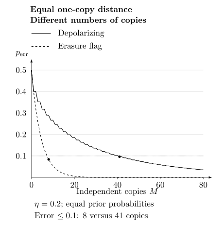
Independent copies, equal priors and $\eta=0.2$. Both channels have one-copy error $0.4$, but error at most $0.1$ requires eight erasure-channel outputs versus 41 depolarizing-channel outputs. The curves show exact binomial and all-erased probabilities, not a fitted asymptotic law.

Rescaling an attenuated expectation

Suppose a measured variable $Y$ has $\mathbb E Y=\eta\mu$ and variance $v$. If $\eta$ is known, the estimator $\hat\mu=\sum_iY_i/(M\eta)$ is unbiased and has

$$\operatorname{Var}(\hat\mu)=\frac{v}{M\eta^2}.$$

With $v\le1$, taking $M\ge1/(\eta^2\epsilon^2)$ is sufficient for standard error at most $\epsilon$. An upper bound on variance supplies a sufficient sample count, not a necessary lower bound. A lower bound on the actual variance or a statistical impossibility theorem is needed for necessity. Standard error is also different from a specified tail-confidence guarantee.

For depolarized Pauli measurements, $v=1-\eta^2\mu^2$. If calibration uses $\hat\eta$ instead of the true $\eta$, the bias is $(\eta/\hat\eta-1)\mu$ and need not vanish as $M\to\infty$. Correlations between shots invalidate the independent-sample variance formula.

Mitigation and error correction

Formal mitigation bounds retain the noise channel, estimator class and circuit-family assumptions. Takagi and collaborators prove sampling-cost limitations for broad protocols; Tsubouchi and collaborators treat unbiased estimation through quantum estimation theory; Quek and collaborators establish stronger worst-case limitations for particular noisy circuit families Takagi et al. (2022), Tsubouchi et al. (2023), Quek et al. (2024).

Postselection can improve conditional quality when the accepted event is informative, but need not do so for an arbitrary filter. Its rejected runs still consume resources. See limits of error mitigation, zero-noise extrapolation and probabilistic cancellation.

A bound for a specified mitigation model is not a contradiction of a fault-tolerance theorem. Encoding, syndrome extraction and active recovery change the allowed implementation. Threshold results then have their own noise, control and resource assumptions.

Oracle separations and physical implementations

The ordinary relations BPP versus BQP and NP versus BQP remain unresolved. An oracle separation answers a different, precise question. Bennett and collaborators show that a uniformly random oracle separates NP from BQP with probability one; Raz and Tal construct an oracle with $\mathrm{BQP}^O\not\subseteq\mathrm{PH}^O$ Bennett et al. (1997), Raz and Tal (2022). Deleting the oracle superscript would change each theorem.

Such results rule out a containment proof that would remain valid uniformly relative to every oracle. They do not rule out a nonrelativizing proof, nor provide a cheap physical implementation of the oracle. Quantum complexity classes develops the definitions and known containments.

A worked conversion from calls to an executed circuit

Suppose a chosen program makes $40$ oracle calls, arranged in ten serial rounds of four parallel calls. The implementation uses $800$ gates per call and depth $120$ per round, with enough separate resources for that parallelism. Other work takes $12{,}000$ gates and depth $900$. Assuming these counts include routing and cleanup without overlap, one attempt uses

$$G=44{,}000, \qquad D=2{,}100.$$

If the component counts are upper bounds, these are upper bounds too, rather than exact identities. The gate count alone does not specify depth, and logical depth does not specify seconds.

Suppose attempts are independent and a correctly recognizable success occurs with probability $3/4$. Four attempts give at least $99\%$ probability of obtaining a success, since $1-(1/4)^4=255/256\approx0.996094$. Sequential execution has worst-case budget $176{,}000$ gates and depth $8{,}400$. Stopping after the first verified success lowers the expected cost; it does not change that budget.

If success is not recognizable, this calculation only says a correct answer appears somewhere in the list. It does not tell us which answer to return. Decision problems may permit majority voting; estimates may require confidence intervals or validation. No such rule follows from the per-attempt success number alone.

Resource estimation adds physical code cycles, device timing and control constraints; algorithmic benchmarking compares executed workloads. Neither step is supplied by an oracle-query count.

Exercises

1. Restore the quantifiers and normalization

A claim says, “Every sparse Hamiltonian needs at least $\tau/(2\pi)$ gates to simulate.” Rewrite the original no-fast-forwarding conclusion using $\sigma=\lVert H\rVert |t|$, and explain why a fixed matrix cannot be declared hard for every specialized query procedure.

Solution

For each size $N$, the two-sparse oracle family has $\sigma=\pi N/2$. Every algorithm simulating all its members to the specified trace-distance accuracy needs at least $N/4$ Hamiltonian queries in the worst case. The hard input may depend on the algorithm. The statement counts queries, uses $\sigma$ rather than the distinct sparse-entry $\tau$, and does not assert hardness of all structured inputs. A known individual instance can have its answer or target transformation built into a specialized procedure; the lower bound concerns unknown members of the family.

2. Count generic state parameters

In an exact ancilla-free circuit with arbitrary one-qubit gates and CNOTs, an initial product state has $2n$ real parameters and each CNOT can expose at most four additional independent parameters after local redundancies are removed. Derive a necessary generic CNOT count and evaluate it for $n=3$. Is it sufficient?

Solution

Matching $2^{n+1}-2$ parameters requires

$$k\ge\left\lceil\frac{2^n-n-1}{2}\right\rceil.$$

For $n=3$ this gives $k\ge2$. Counting supplies a necessary condition, not a construction proving sufficiency. It applies to almost all exact states in the specified circuit model, and does not exclude short preparations of special states or establish an approximation bound.

3. Identify the information absent from a state

An algorithm prepares the normalized state proportional to $x=(1,i,2)$ and estimates a specified observable. Can state copies distinguish $x$ from $x'=-3i\,x$? What extra choices are needed for an explicit classical-vector output?

Solution

The two vectors give the same normalized density operator $xx^\dagger/\lVert x\rVert^2$. No measurement on any number of copies can distinguish them. Recovering an unnormalized vector needs separate norm information and a global-phase convention. Even then, reconstructing every coordinate is a larger task than estimating one observable, and writing the finite-precision result requires its output bits.

4. Include data preparation and reuse

For $B_Q=1000$, $B_C=100$, $U_Q=2$ and $U_C=5$, find the integer reuse counts for which the quantum total is strictly smaller. Then suppose quantum data must be rebuilt before every use.

Solution

The comparison $1000+2R<100+5R$ gives $R>300$, so the first integer is $301$. With rebuilding, quantum cost becomes $1002R$, exceeding $100+5R$ for every integer $R\ge1$ in this example. Preprocessing can be amortized only when the workload really permits reuse.

5. Separate variance, confidence and calibration

Let $\eta=0.2$, $v\le1$ and target standard error $\epsilon=0.02$. Find a sufficient sample count for independent rescaled measurements. If $\mu=0.5$ but the calibration uses $\hat\eta=0.22$, find the limiting bias. Does taking more samples remove it?

Solution

The variance bound gives $M\ge1/[(0.2)^2(0.02)^2]=62{,}500$, compared with $2500$ at unit attenuation. These are sufficient worst-case standard-error counts for this estimator, not a universal necessity or a tail-confidence statement. The limiting bias is $(0.2/0.22-1)(0.5)=-1/22\approx-0.045455$. More independent shots reduce variance but leave this systematic bias.

6. Interpret an oracle separation

Does $\exists O:\mathrm{BQP}^O\not\subseteq\mathrm{PH}^O$ prove $\mathrm{BQP}\not\subseteq\mathrm{PH}$, or prove that no classical circuit can implement the separating oracle efficiently?

Solution

Neither follows. The theorem treats queries to $O$ as supplied operations and concerns the relativized classes. It excludes a uniformly relativizing BQP-within-PH argument, but the unrelativized relation and ordinary implementation cost require additional results.

7. Budget repetitions and recognize success

Use the $44{,}000$-gate, depth-$2100$ attempt above. Verify that four independent attempts are necessary for at least $99\%$ probability of some recognizable success. Find the expected number executed when stopping at the first success, with a four-attempt cap.

Solution

Three attempts succeed with probability $1-1/64=0.984375$; four give $255/256$. The expected count under the stopping rule is

$$1+\frac14+\frac1{16}+\frac1{64} =\frac{85}{64}=1.328125.$$

Expected gates are $58{,}437.5$ and expected sequential depth is $2789.0625$ in this simplified model, versus budgets $176{,}000$ and $8400$. Actual time still requires timing information. If success cannot be recognized, the stopping rule is unavailable: a list containing a correct answer is not automatically an identified correct answer.

References

• S. Aaronson, “Shadow Tomography of Quantum States,” SIAM Journal on Computing 49(5), STOC18-368–STOC18-394 (2020), doi:10.1137/18M120275X.
• Y. Atia and D. Aharonov, “Fast-Forwarding of Hamiltonians and Exponentially Precise Measurements,” Nature Communications 8, 1572 (2017), doi:10.1038/s41467-017-01637-7.
• C. H. Bennett, E. Bernstein, G. Brassard, and U. Vazirani, “Strengths and Weaknesses of Quantum Computing,” SIAM Journal on Computing 26, 1510–1523 (1997), doi:10.1137/S0097539796300933.
• D. W. Berry, G. Ahokas, R. Cleve, and B. C. Sanders, “Efficient Quantum Algorithms for Simulating Sparse Hamiltonians,” Communications in Mathematical Physics 270, 359–371 (2007), doi:10.1007/s00220-006-0150-x.
• D. W. Berry, A. M. Childs, and R. Kothari, “Hamiltonian Simulation with Nearly Optimal Dependence on All Parameters,” in Proceedings of the 56th IEEE Annual Symposium on Foundations of Computer Science, 792–809 (2015), doi:10.1109/FOCS.2015.54.
• N.-H. Chia, A. Gilyén, T. Li, H.-H. Lin, E. Tang, and C. Wang, “Sampling-Based Sublinear Low-Rank Matrix Arithmetic Framework for Dequantizing Quantum Machine Learning,” in Proceedings of the 52nd Annual ACM Symposium on Theory of Computing, 387–400 (2020), doi:10.1145/3357713.3384314.
• V. Giovannetti, S. Lloyd, and L. Maccone, “Quantum Random Access Memory,” Physical Review Letters 100, 160501 (2008), doi:10.1103/PhysRevLett.100.160501.
• J. Haah, A. W. Harrow, Z. Ji, X. Wu, and N. Yu, “Sample-Optimal Tomography of Quantum States,” IEEE Transactions on Information Theory 63, 5628–5641 (2017), doi:10.1109/TIT.2017.2719044.
• A. W. Harrow, A. Hassidim, and S. Lloyd, “Quantum Algorithm for Linear Systems of Equations,” Physical Review Letters 103, 150502 (2009), doi:10.1103/PhysRevLett.103.150502.
• A. Lowe and A. Nayak, “Lower Bounds for Learning Quantum States with Single-Copy Measurements,” ACM Transactions on Computation Theory 17(1), Article 7, 42 pages (2025), doi:10.1145/3717450.
• A. Nayak, “Optimal Lower Bounds for Quantum Automata and Random Access Codes,” in Proceedings of the 40th Annual Symposium on Foundations of Computer Science, 369–376 (1999), doi:10.1109/SFFCS.1999.814608.
• Y. Quek, D. Stilck França, S. Khatri, J. J. Meyer, and J. Eisert, “Exponentially Tighter Bounds on Limitations of Quantum Error Mitigation,” Nature Physics 20, 1648–1658 (2024), doi:10.1038/s41567-024-02536-7.
• R. Raz and A. Tal, “Oracle Separation of BQP and PH,” Journal of the ACM 69(4), Article 30 (2022), doi:10.1145/3530258.
• V. V. Shende, S. S. Bullock, and I. L. Markov, “Synthesis of Quantum-Logic Circuits,” IEEE Transactions on Computer-Aided Design of Integrated Circuits and Systems 25, 1000–1010 (2006), doi:10.1109/TCAD.2005.855930.
• R. Takagi, S. Endo, S. Minagawa, and M. Gu, “Fundamental Limits of Quantum Error Mitigation,” npj Quantum Information 8, 114 (2022), doi:10.1038/s41534-022-00618-z.
• E. Tang, “A Quantum-Inspired Classical Algorithm for Recommendation Systems,” in Proceedings of the 51st Annual ACM Symposium on Theory of Computing, 217–228 (2019), doi:10.1145/3313276.3316310.
• K. Tsubouchi, T. Sagawa, and N. Yoshioka, “Universal Cost Bound of Quantum Error Mitigation Based on Quantum Estimation Theory,” Physical Review Letters 131, 210601 (2023), doi:10.1103/PhysRevLett.131.210601.