Quantum Linear Algebra

The quantum linear-systems problem asks for useful information about the solution of $Ax=b$ when the coefficient matrix and right-hand side are exposed through specified coherent interfaces. For an invertible matrix, its standard quantum output is the normalized state

$$\lvert x\rangle := \frac{A^{-1}\lvert b\rangle} {\lVert A^{-1}\lvert b\rangle\rVert_2},$$

not a classical list of the entries of $x$. This distinction is decisive: a state can support selected observables, overlaps, samples, or a subsequent coherent computation, but reading all $N$ complex coordinates has an $\Omega(N)$-scale description burden even before precision is counted.

The central difficulty is to apply an inverse while respecting quantum normalization. Small singular values magnify some input components, so implementing the inverse requires a scale factor and a success procedure. This page derives those steps, explains the role of conditioning, and compares the main algorithms under their stated matrix and input-state access.

Helpful background. Quantum phase estimation explains coherent spectral labels; Hamiltonian simulation algorithms supplies the controlled evolution used in HHL. Singular-value decomposition is useful for non-Hermitian and rectangular systems.

The Quantum Linear-Systems Problem

Begin with a finite-dimensional system

$$Ax=b, \qquad A\in\mathbb C^{N\times N}, \qquad b\ne0.$$

The data vector and the solution must be normalized separately:

$$\lvert b\rangle := \frac{b}{\lVert b\rVert_2}, \qquad \lvert x\rangle := \frac{A^{-1}\lvert b\rangle} {\lVert A^{-1}\lvert b\rangle\rVert_2}.$$

Multiplying $b$ by a nonzero complex scalar changes the normalized vectors only by a global phase, so it does not change their physical states. Also, the solution-state output does not reveal $\lVert A^{-1}b\rVert_2$. A global phase is also unobservable. These facts make QLSP a state-preparation problem, not ordinary classical linear algebra with a different storage format.

If $N$ is not a power of two, use $n=\lceil\log_2N\rceil$ qubits and embed the system in a $2^n$-dimensional register. The algorithm must protect the unused subspace—for example, by defining an invertible extension with a separated spectrum and ensuring that preparation has no support on the padding basis states. Merely appending zero rows and columns would make the extended matrix singular and change the problem promise.

For pure-state output, we use the phase-aligned Euclidean guarantee

$$\min_{\varphi\in\mathbb R} \left\lVert \lvert\widetilde x\rangle -e^{i\varphi}\lvert x\rangle \right\rVert_2 \leq\epsilon,$$

conditional on a declared herald. An implementation with residual entanglement can instead produce a mixed state, requiring a trace-distance or fidelity guarantee; one cannot assign it a single output ket. A theorem must also give the heralding probability or adopt a stated constant-success convention and charge the amplification or repetition used to reach it. This metric is not interchangeable with a residual $\lVert A\widetilde x-b\rVert_2$, an operator error, infidelity, observable error, or entrywise classical error. Any translation needs its own inequality and hypotheses.

For a singular or rectangular matrix, $A^{-1}$ is not available. One must instead declare a singular-value cutoff, the input support, and whether the task prepares a truncated-pseudoinverse state or solves a specified least-squares problem. In particular, an inconsistent equation may not be silently redefined by projecting $b$ onto the column space.

Matrix, Right-Hand-Side, and Block-Encoding Access

The right-hand side enters through a declared unitary

$$U_b\lvert0^n\rangle=\lvert b\rangle.$$

Whether $U_b^\dagger$ and controlled $U_b$ are available must be stated. An already-prepared copy of $\lvert b\rangle$ is weaker than a repeatable unitary: it cannot automatically be inverted to implement a reflection or coherently embedded in amplitude amplification. A classical array, a QRAM data structure, an amplitude-preparation circuit, and sample/query access likewise represent different inputs. Their setup time, update rules, precision, memory, and reversibility can dominate the advertised query count.

A block encoding makes one matrix interface precise. An $(\alpha,a,\epsilon_A)$ block encoding is a unitary $U_A$ on $a+n$ qubits such that $\alpha\geq\lVert A\rVert_2$ and

$$\left\lVert A- \alpha (\langle0^a\rvert\otimes I) U_A (\lvert0^a\rangle\otimes I) \right\rVert \leq\epsilon_A.$$

The scaling $\alpha$, ancilla width $a$, and block error $\epsilon_A$ are part of the input contract. So are calls to $U_A^\dagger$, controlled calls, and the reflection about the signal ancillas. A block query may expand into many sparse-oracle calls, selected unitaries, arithmetic operations, or memory lookups; the appropriate conversion theorem and its error must be charged.

Sparse access instead often supplies coherent position and value oracles. A row index and an integer label identify a possible nonzero position, and a second reversible operation writes a finite-precision entry. The model needs a sparsity bound, a convention for duplicates or padding, and access to rows and columns where the reduction requires both. A formula for $A_{jk}$ or a promise that $A$ is sparse does not implement either oracle. Similarly, a sum of unitaries, controlled Hamiltonian evolution, and a projected-unitary encoding are not interchangeable names for access.

The quantum oracles page explains these interface distinctions. For an implementation, expand each query into its reversible computation or data lookup, including ancillas, precision and controls. If a location oracle overwrites its index, its padded location list must be injective and have a reversible extension.

Conditioning, Scaling, and Spectral Promises

For an invertible matrix, the intrinsic spectral condition number is

$$\kappa_2(A) := \lVert A\rVert_2\lVert A^{-1}\rVert_2 = \frac{\sigma_{\max}(A)}{\sigma_{\min}(A)}.$$

This quantity describes sensitivity of the mathematical inverse in the spectral norm. An access model introduces additional scaling. Choose and declare an inverse normalization

$$\alpha_{A^{-1}} \geq \lVert A^{-1}\rVert_2$$

and define the block condition number

$$\kappa_{\mathrm{block}} := \alpha\alpha_{A^{-1}} \geq \kappa_2(A).$$

For an exact invertible instance with tight inverse normalization, $\alpha_{A^{-1}}=1/\sigma_{\min}(A)$ and therefore $\kappa_{\mathrm{block}}=\alpha/\sigma_{\min}(A)$. Over-normalizing the same matrix can enlarge this access-induced parameter without changing $\kappa_2(A)$ or the normalized solution state. It should not be renamed an “effective condition number”: that phrase is also used for an instance- and tolerance-dependent spectral-truncation quantity.

The matching instance amplitude is

$$p_b := \frac{ \lVert A^{-1}\lvert b\rangle\rVert_2^2 }{ \alpha_{A^{-1}}^2 }.$$

It can be much larger than its worst-case lower bound, and modern two-oracle results exploit that distinction. A theorem using a loose but proved $\alpha_{A^{-1}}$ must retain the same normalization in both $p_b$ and $\kappa_{\mathrm{block}}$.

Representation error can be amplified by inversion. If $\lVert E\rVert<\sigma_{\min}(A)$, the resolvent identity gives the exact perturbation bound

$$\left\lVert (A+E)^{-1}-A^{-1} \right\rVert \leq \frac{ \lVert E\rVert }{ \sigma_{\min}(A) \left[ \sigma_{\min}(A)-\lVert E\rVert \right] }.$$

Thus block-encoding error, right-hand-side preparation error, reciprocal or polynomial approximation, Hamiltonian simulation, phase or gate synthesis, and final measurement need separate budgets. A small residual does not by itself imply a small forward error for an ill-conditioned system, and even a forward-vector bound needs normalization control before it implies the state metric used here. Conditioning and Stability develops those general numerical distinctions.

There is a useful normalization inequality. If $y\ne0$, $\widetilde y\ne0$ and $\|\widetilde y-y\|\leq\eta$, then

$$\left\|\frac{\widetilde y}{\|\widetilde y\|} -\frac{y}{\|y\|}\right\| \leq\frac{2\eta}{\|y\|}.$$

Insert $\widetilde y/\|y\|$ between the two normalized vectors and use $|\|\widetilde y\|-\|y\||\leq\eta$. In particular, an implemented inverse block $F$ approximating $cA^{-1}$ to operator error $\eta$ gives a normalized-state error at most $2\eta/(|c|\|A^{-1}|b\rangle\|)$, provided its output is nonzero. A small successful branch therefore needs a tighter absolute block error.

HHL as a Spectral Inversion Procedure

The historical HHL construction is clearest for Hermitian $A$, rescaled so that $\lVert A\rVert_2=1$. In this specialization only, write

$$\kappa := \kappa_2(A) = \lVert A^{-1}\rVert_2,$$

so the supported eigenvalues obey

$$\lambda_j \in [-1,-1/\kappa]\cup[1/\kappa,1], \qquad \lvert b\rangle = \sum_j\beta_j\lvert u_j\rangle.$$

Controlled evolution and phase estimation coherently label each eigenvalue. Choose the phase scale so that positive and negative eigenvalues are distinguishable modulo one; the promised spectral gap excludes the singular point. In the ideal exact-label description, a flag rotation with $0<C\leq1/\kappa$ gives

$$\sum_j\beta_j|u_j\rangle|\lambda_j\rangle \left(\sqrt{1-C^2/\lambda_j^2}|0\rangle +\frac{C}{\lambda_j}|1\rangle\right).$$

The sign of $\lambda_j$ must remain in the flag-one amplitude. At this stage the eigenvalue register is still present and correlated with the system. Reversing the exact labeling operation resets it to $|0\rangle$, after which the flag-one branch is

$$C\sum_j\frac{\beta_j}{\lambda_j}|u_j\rangle =CA^{-1}|b\rangle.$$

Discarding the label instead of uncomputing it generally destroys the desired coherence. For example, the diagonal two-level calculation below would then give a mixture rather than $(|0\rangle+2|1\rangle)/\sqrt5$. Actual finite phase estimation uses a superposition of estimates rather than exact labels, so the reciprocal approximation and uncomputation errors must be analyzed together. The ideal expression explains the mechanism; it is not an exact description of a finite-resolution implementation.

Finite phase estimation matters because the reciprocal is steep near the spectral gap. If $|\widetilde\lambda-\lambda|\leq\delta_\lambda$, $|\lambda|\geq1/\kappa$, and $\delta_\lambda\leq1/(2\kappa)$, then $|\widetilde\lambda|\geq1/(2\kappa)$ and

$$\left| \frac{1}{\widetilde\lambda} - \frac{1}{\lambda} \right| = \frac{|\widetilde\lambda-\lambda|} {|\widetilde\lambda\lambda|} \leq 2\kappa^2\delta_\lambda.$$

This elementary check connects eigenvalue precision to reciprocal error, but it is not a full output proof. Simulation, phase estimation, reversible arithmetic, rotation synthesis, uncomputation, postselection, and normalization must fit one state-error budget. Harrow, Hassidim, and Lloyd’s 2009 result established the paradigm under efficient sparse access and state preparation; its historical precision dependence should not be presented as the best modern bound.

Success Probability, Amplification, and Variable Time

The ideal flag probability follows directly from the branch norm:

$$p_C = C^2 \left\lVert A^{-1}\lvert b\rangle \right\rVert_2^2.$$

Choosing $C=1/\alpha_{A^{-1}}$ makes $p_C=p_b$. With tight normalization this is $C=1/\lVert A^{-1}\rVert_2=\sigma_{\min}(A)$. Plain repetition therefore uses $O(1/p_C)$ complete state-preparation attempts in expectation. Coherent Amplitude Amplification can reduce the dependence to $O(1/\sqrt{p_C})$, but only if the full preparation and its inverse, the success test, and the needed reflections and controls are executable. A copy of a prepared input state does not supply that contract.

With tight $C=\sigma_{\min}(A)$, the ideal probability lies in $[1/\kappa_2(A)^2,1]$. Its minimum occurs when $|b\rangle$ is a left singular vector with the largest singular value; its maximum occurs at the smallest singular value. For a Hermitian matrix these are eigenvectors ordered by eigenvalue magnitude. Small eigenvalues create the difficult spectral-resolution scale, but they receive larger inverse amplitudes. These are distinct effects; conditioning alone does not specify the actual heralding probability. Variable-time algorithms partition branches according to the precision or evolution time they require, stop well-resolved branches early, and amplify a procedure with multiple stopping times. Ambainis’s 2012 analysis improved the isolated historical dependence from $O(\kappa^2\log N)$ to $O(\kappa\log^3\!\kappa\log N)$ in its model. That statement neither supplies a modern precision-resolved end-to-end runtime nor makes early stopping, clocks, inverse operations, or state preparation free.

Success probability and approximation error answer different questions. One can have a highly accurate conditional branch that is almost never observed, or a constant-probability branch implementing a poor reciprocal. A complete solver fixes both, allocates an allowed failure probability, and says whether the reported cost is an average, a worst-case cap, or an expected number of attempts.

Polynomial, Fourier, and QSVT Linear Solvers

Later methods replace a high-precision binary eigenvalue register by a direct approximation to the reciprocal on a promised spectral domain. Childs, Kothari, and Somma construct Fourier- and Chebyshev-based linear combinations in a sparse-access model, obtaining polylogarithmic rather than polynomial dependence on $1/\epsilon$ after the full success procedure is included. Gilyén, Su, Low, and Wiebe formulate singular-value transformation, which applies an admissible polynomial to the singular values exposed by a projected unitary encoding. Lin and Tong use polynomial filtering and a Zeno-style construction, while Subaşı, Somma, and Orsucci develop a randomized-adiabatic family. These methods share a spectral-inversion goal, not a single access or resource theorem.

To state the QSVT inverse clearly, write $\bar A=A/\alpha$ and suppose its supported singular values lie in $[\delta,1]$. The conventional bounded transform approximates

$$\frac{\delta}{2}\bar A^+ =\frac{\delta\alpha}{2}A^+$$

to operator error $\eta$, using $O(\delta^{-1}\log(1/\eta))$ encoded-operator calls. If $\delta=1/\kappa_{\mathrm{block}}$, its scale is $A^+/(2\alpha_{A^{-1}})$. The factor $1/2$ is part of this polynomial construction, not the maximal allowed HHL flag amplitude. The normalization inequality above translates $\eta$ into a solution-state tolerance before amplification costs are assigned.

For $A=U\Sigma V^\dagger$, pseudoinversion must map the left singular vectors to the right ones: $A^+=V\Sigma^+U^\dagger$. Applying an odd singular-value transform in the forward $U\!\leftarrow\!V$ direction instead produces $U f(\Sigma)V^\dagger$, which has the wrong orientation for a general non-Hermitian inverse. Use the adjoint encoding or reverse the projected input/output spaces. Block encodings and QSVT develops that construction and its polynomial constraints. Singular problems also need a gap or transition interval around the chosen cutoff; a finite polynomial cannot uniformly implement a discontinuous sharp cutoff across arbitrary singular values.

Comparing calls to the matrix and input preparation

The following representative bounds have different assumptions. In the sparse rows, $A$ is Hermitian with $\|A\|=1$, condition bound $\kappa$, at most $d$ entries per row and column, reversible sparse access and repeatable preparation $P_B|0\rangle=|b\rangle$. In the block rows, the normalized matrix, input preparation, inverses and necessary controlled operations are supplied. State-output rows include a constant-success procedure; readout and construction of the supplied operations remain additional.

Method	Representative cost	What the bound describes
HHL	Historical $\widetilde O(d^2\kappa^2\log N/\epsilon)$ runtime	Sparse controlled simulation, phase estimation and amplification in the original model; not a classical vector output.
Fourier/Chebyshev with variable time	$O(d\kappa\,\mathrm{polylog}(d\kappa/\epsilon))$ calls to each sparse/input oracle	Childs–Kothari–Somma state preparation, with its reversible variable-time construction.
QSVT inverse transform	$O(\delta^{-1}\log(1/\eta))$ block calls	An operator approximation to the scaled inverse; input preparation and amplification are still needed.
Discrete adiabatic solver	$O(\kappa\log(1/\epsilon))$ average oracle calls	Costa and collaborators’ supplied-block state-output theorem, with its normalization and constant-success convention.

For a sharper separation of the two inputs, Low and Su give a tunable variable-time construction. With a constant-factor estimate of $\|A^{-1}|b\rangle\|$ supplied, define $L=\max\{1,\log(p_b^{-1/2})\}$. Their theorem gives

$$Q_b=O(p_b^{-1/2}), \qquad Q_A=O\!\left(\kappa_{\mathrm{block}}L \log\frac{L}{\epsilon}\right).$$

Here $Q_b$ counts initial-state operations and $Q_A$ counts block operations, including the required adjoints and controls. The preparation dependence is worst-case optimal in the paper’s tight inverse-normalization convention. The explicit maximum avoids interpreting a logarithm at $p_b=1$ as zero cost. If the norm estimate is not supplied, obtaining it is a separate step: the paper preserves the optimal preparation scaling, but its matrix-query cost must also be included. One cannot quote the displayed two-oracle bound unconditionally. These bounds distinguish oracle uses, not physical runtime; a cheap matrix oracle and expensive state preparation may favor a different algorithm from the converse situation.

Non-Hermitian, Rectangular, and Least-Squares Problems

HHL’s Hermitian presentation is not a license to discard non-Hermitian structure. For an invertible square matrix, one standard reduction uses the Hermitian dilation

$$\mathcal A := \begin{pmatrix} 0&A\\ A^\dagger&0 \end{pmatrix}.$$

With compatible ordering of the two block registers,

$$\mathcal A^{-1} \begin{pmatrix} b\\0 \end{pmatrix} = \begin{pmatrix} 0\\A^{-1}b \end{pmatrix}.$$

The nonzero eigenvalue magnitudes of $\mathcal A$ are the singular values of $A$, so this dilation preserves the intrinsic spectral condition number. It does not preserve every implementation constant for free. The register is larger, access to $A^\dagger$ is required, a block or sparse interface for $\mathcal A$ must be constructed, and its normalization, sparsity convention, controls, and precision enter the operation count and error bound.

For a rectangular matrix with singular-value decomposition $A=U\Sigma V^\dagger$, the input and output inhabit different singular-vector spaces. With cutoff $\delta>0$, define

$$A_\delta^+ := \sum_{\sigma_j\geq\delta} \frac{1}{\sigma_j} \lvert v_j\rangle\langle u_j\rvert.$$

The right-hand side is supplied in the left-singular space and the output is proportional to $A_\delta^+\lvert b\rangle$ in the right-singular space. A component of $b$ below the cutoff or outside the column space must be handled explicitly: reject it as invalid input, project it and disclose the lost norm, or define a least-squares objective whose minimizer uses that projection. The cutoff causes bias, changes the success amplitude, and sets the relevant condition parameter. Singular-value decomposition develops the pseudoinverse and its minimum-norm least-squares interpretation.

Regularization changes the task again. Replacing $1/\sigma$ by, for example, $\sigma/(\sigma^2+\mu)$ can suppress unstable small singular values, but the output is then a regularized solution state. Its approximation interval, regularization bias, normalization, and downstream statistic must be stated; it is not an exact QLSP with a mysteriously improved condition number.

Outputs, Observables, and Readout

The solution register is useful when the application can remain quantum or asks for a low-dimensional functional. If $M$ is a bounded observable, a natural target is

$$\mu_M := \langle x\rvert M\lvert x\rangle.$$

For phase-aligned unit vectors separated by at most $\epsilon$, the preparation contribution obeys the simple bound

$$\left| \langle\widetilde x\rvert M\lvert\widetilde x\rangle - \langle x\rvert M\lvert x\rangle \right| \leq 2\lVert M\rVert\epsilon.$$

Statistical error is additional. If $M$ is measured with outcomes in $[-1,1]$, ordinary independent sampling uses fresh successful preparations; Hoeffding’s inequality gives a sufficient shot count $m\geq2\ln(2/\eta)/\delta^2$ for additive statistical error $\delta$ and failure probability at most $\eta$. Each shot therefore expands to another preparation, herald check, and possible retry. Coherent amplitude-estimation improvements require a repeatable preparation unitary, its inverse, reflections, and controlled uses, so they invoke a stronger access contract than independent samples.

A computational-basis measurement yields one index distributed according to $|x_j|^2$; it does not reveal phases, normalization of the unnormalized solution, or all coordinates. Tomography or dense classical output inherits an $\Omega(N)$-scale description requirement before accuracy and confidence are included. A meaningful application should instead name the overlap, expectation, sample, threshold decision, or subsequent coherent transformation that consumes $\lvert x\rangle$.

See lower bounds and limitations for the general input-loading and explicit-output costs.

Verification is not automatic either. In the black-box model analyzed by Somma and Subaşı, constant-distance coherent verification requires $\Omega(\kappa)$ uses of $U_b$, $U_b^\dagger$, or controlled variants in the worst case and typically $\Omega(\sqrt\kappa)$. A prepare-and-measure strategy requires $\Omega(\kappa^2)$ copies in the worst case and typically $\Omega(\kappa)$. Special structure can provide a cheaper residual, energy, observable, or application-specific certificate, but its measurement and the inequality linking it to the desired state guarantee must be supplied. Preparing a candidate does not certify it.

Complexity Bounds and Matched Classical Comparisons

Dimension, conditioning, precision, sparsity, input overlap, and success are independent asymptotic variables. A statement that is polylogarithmic in $N$ may still be polynomial in $\kappa$, $1/\epsilon$, sparsity, or inverse success amplitude. It may also count only ideal oracle calls. Query Complexity explains upper bounds, reductions and oracle lower bounds; the QLSP results must retain their particular access models.

In the block-encoding parity-reduction regime, a proved lower bound requires

$$\Omega\!\left( \kappa\log\frac{1}{\epsilon} \right)$$

encoded-matrix queries. It matches the joint condition-and-precision scaling of the discrete-adiabatic upper bound within that oracle setting. Mori, Kikuchi, Benedetti, and Rosenkranz proved a different 2026 lower bound, $\Omega(\kappa\sqrt{s})$, for sparse queries at constant error. These bounds cannot be multiplied or merged: their interfaces and error regimes differ. These two theorems alone do not establish a product $\Omega(\kappa\sqrt{s}\log(1/\epsilon))$ bound. Dated questions about sharper tradeoffs are discussed in query-complexity frontiers. Neither query result is a universal gate-count, circuit-depth, physical- runtime, or wall-clock lower bound.

Classical comparison begins by matching the task. The conjugate-gradient method introduced by Hestenes and Stiefel is a natural comparator for sparse Hermitian positive-definite systems when a classical vector is wanted. Its iteration behavior depends on conditioning, while each iteration charges a sparse matrix–vector product and classical vector operations. That is not the same output contract as preparing $\lvert x\rangle$. Conversely, comparing a quantum state-output theorem only with the cost of printing a classical dense vector can manufacture a separation by requiring the classical method to solve a stronger problem.

The Classical Information Review supplies the representation and access matching needed here. A dense-memory quantum interface or length-square sample/query access may require substantial preprocessing and can enable stronger classical algorithms too. The comparison must therefore use the same matrix data structure, update model, right-hand-side access, condition and rank promises, output functional, accuracy, confidence, preprocessing, memory, and hardware boundary.

For an application, add the costs of constructing the oracles, compiling their controlled and inverse operations, and extracting the requested observable. Algorithmic benchmarking explains how to compare such complete computations; resource estimation tools connects logical operations to a proposed implementation. Polylogarithmic dimension dependence in a supplied-oracle theorem alone establishes no generic exponential advantage.

Two diagonal systems

Reciprocal weighting changes the state direction

Take

$$A = \operatorname{diag}\!\left(1,\frac12\right), \qquad \lvert b\rangle = \frac{\lvert0\rangle+\lvert1\rangle}{\sqrt2}, \qquad C=\frac12.$$

Then

$$\kappa_2(A)=2, \qquad A^{-1}\lvert b\rangle = \frac{\lvert0\rangle+2\lvert1\rangle}{\sqrt2}, \qquad \lvert x\rangle = \frac{\lvert0\rangle+2\lvert1\rangle}{\sqrt5}.$$

The two reciprocal-rotation flag amplitudes are $1/2$ and $1$, so

$$p_C = \frac12 \left[ \left(\frac12\right)^2+1^2 \right] = \frac58.$$

quantity	exact value	interpretation
$\kappa_2$	$2$	intrinsic condition number
flag amplitude for $\lambda=1$	$1/2$	$C/\lambda$ on $\lvert0\rangle$
flag amplitude for $\lambda=1/2$	$1$	$C/\lambda$ on $\lvert1\rangle$
$p_C$	$5/8$	ideal herald probability
$P(0)$	$1/5$	postselected computational-basis probability
$P(1)$	$4/5$	postselected computational-basis probability
$\langle Z\rangle$	$-3/5$	one observable, not both coordinates

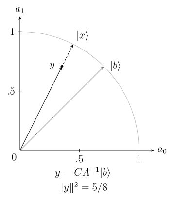
The input has equal components. The filter $CA^{-1}=\operatorname{diag}(1/2,1)$ attenuates the first component, producing a branch of norm $\sqrt{5/8}$. Conditioning on success divides by that norm; the normalized output points along $(1,2)$. The drawn amplitudes are real for this example.

If the exact eigenvalue label were discarded before uncomputation, the same flag probabilities would remain, but the conditional system state would be

$$\rho_{\mathrm{discard}}=\frac15|0\rangle\langle0|+\frac45|1\rangle\langle1|.$$

It has $\langle X\rangle=0$, whereas the intended pure solution has $\langle X\rangle=4/5$. Checking only the two basis probabilities or $\langle Z\rangle$ would miss the loss of coherence.

Normalization of the matrix encoding changes the cost

Now take

$$A = \operatorname{diag}\!\left(1,\frac14\right), \qquad \lvert b\rangle = \frac{\lvert0\rangle+\lvert1\rangle}{\sqrt2}, \qquad \alpha_{A^{-1}}=4 \quad\text{(tight)}.$$

Exact inversion gives

$$\kappa_2(A)=4, \qquad \lvert x\rangle = \frac{\lvert0\rangle+4\lvert1\rangle}{\sqrt{17}}, \qquad p_b = \frac{17}{32}.$$

quantity	exact value	interpretation
$\kappa_2$	$4$	intrinsic condition number
$p_b$	$17/32$	tight HHL-style success with $C=1/4$
$P(0)$	$1/17$	one basis probability
$P(1)$	$16/17$	the other basis probability
$\langle Z\rangle$	$-15/17$	selected observable output
block condition number for $\alpha=1$	$4$	tight matrix normalization
block condition number for $\alpha=2$	$8$	over-normalized access to the same $A$

The HHL-style scale $C=1/4$ produces success $17/32$. By contrast, the conventional QSVT pseudoinverse theorem applies the extra factor $1/2$ to the encoded inverse. For $\delta=1/4$ and tight $\alpha=1$, the implemented scale is $A^{-1}/8$, so its unamplified success is $17/128$. Combining that transform with the larger HHL success probability would mix two normalization conventions.

The two encodings have the same normalized solution, yet the looser encoding has a smaller singular-value gap. Conversely, the two inverse-filter scales have different success probabilities even though both successful branches point along the same solution. Distinguishing these effects is essential before comparing algorithm costs.

The following NumPy calculation reproduces both solution states and their ideal HHL-style herald probabilities. It also checks the original equation before normalizing its solution.

import numpy as np

b = np.array([1., 1.]) / np.sqrt(2)
for small in [.5, .25]:
    A = np.diag([1., small])
    y = np.linalg.solve(A, b)
    assert np.allclose(A @ y, b)
    x = y / np.linalg.norm(y)
    success = np.linalg.norm(small * y)**2
    print(x, success, abs(x[0])**2 - abs(x[1])**2)

Exercises

1. Normalize a Quantum Linear-System Instance

Let

$$A=\operatorname{diag}(2,1), \qquad b=\begin{pmatrix}3\\4\end{pmatrix}.$$

Compute $\lvert b\rangle$, the unnormalized vector $A^{-1}\lvert b\rangle$, and the normalized solution state. Explain why solving with $b$ or with $\lvert b\rangle$ produces the same final quantum state but not the same classical solution vector.

Solution

Because $\lVert b\rVert_2=5$,

$$\lvert b\rangle = \frac35\lvert0\rangle+\frac45\lvert1\rangle.$$

Applying the inverse gives

$$A^{-1}\lvert b\rangle = \frac{3}{10}\lvert0\rangle+\frac45\lvert1\rangle, \qquad \left\lVert A^{-1}\lvert b\rangle\right\rVert_2 = \frac{\sqrt{73}}{10}.$$

Therefore

$$\lvert x\rangle = \frac{3\lvert0\rangle+8\lvert1\rangle}{\sqrt{73}}.$$

The classical solutions to $Ax=b$ and $Ax=b/\lVert b\rVert_2$ differ by the factor $5$. Normalization removes that nonzero scalar, so their solution states coincide. The state consequently does not retain the magnitude needed to reconstruct the original classical vector.

2. Derive the HHL Flag Probability

Assume the ideal Hermitian HHL setting with $\lvert b\rangle=\sum_j\beta_j\lvert u_j\rangle$ and flag amplitude $C/\lambda_j$. Derive the heralding probability. Then evaluate it for $A=\operatorname{diag}(1,1/3)$, equal input amplitudes, and $C=1/3$; also give the two postselected basis probabilities.

Solution

Orthogonality of the eigenvectors makes the squared norm of the selected branch

$$p_C = \sum_j \lvert\beta_j\rvert^2 \frac{C^2}{\lvert\lambda_j\rvert^2} = C^2\lVert A^{-1}\lvert b\rangle\rVert_2^2.$$

For the stated instance, the flag amplitudes are $1/3$ and $1$. Hence

$$p_C = \frac12\left(\frac19+1\right) = \frac59.$$

The unnormalized inverse action is proportional to $(1,3)$, so the successful state is $(\lvert0\rangle+3\lvert1\rangle)/\sqrt{10}$. Its basis probabilities are $1/10$ and $9/10$. They require separate successful shots to estimate; the heralding calculation does not output the pair as a classical record.

3. Separate Intrinsic and Block Condition Numbers

Let $A=\operatorname{diag}(1,1/5)$ and use the tight inverse normalization $\alpha_{A^{-1}}=5$. Compare exact block encodings with $\alpha=1$ and $\alpha=3$. Find the intrinsic and block condition numbers, and state what does and does not change for a fixed $\lvert b\rangle$.

Solution

The singular values are $1$ and $1/5$, so

$$\kappa_2(A)=5.$$

The two valid matrix normalizations satisfy $\alpha\geq\lVert A\rVert_2=1$ and give

$$\kappa_{\mathrm{block}}(\alpha=1)=1\cdot5=5, \qquad \kappa_{\mathrm{block}}(\alpha=3)=3\cdot5=15.$$

The matrix, its intrinsic condition number, $A^{-1}\lvert b\rangle$, and its normalized direction are unchanged. The encoded block amplitude and the access-induced condition parameter change. Consequently, a query theorem expressed in $\kappa_{\mathrm{block}}$ can assign different bounds to the two interfaces even though they represent the same mathematical system.

4. Propagate Eigenvalue-Estimation Error

Suppose $\lVert A\rVert_2=1$, $\kappa=5$, an eigenvalue is $\lambda=1/5$, and phase estimation returns $\widetilde\lambda=0.21$. Verify the hypotheses of the reciprocal stability bound, compute the actual reciprocal error, and compare it with the bound. What error sources remain before a state guarantee follows?

Solution

Here $\delta_\lambda=0.01$ and $1/(2\kappa)=0.1$, so the required inequality $\delta_\lambda\leq1/(2\kappa)$ holds. The actual error is

$$\left| \frac{1}{0.21}-5 \right| = \frac{5}{21} \approx0.238095,$$

whereas the elementary bound gives

$$2\kappa^2\delta_\lambda = 2\cdot25\cdot0.01 = 0.5.$$

The bound is valid but not tight for this value. A final state guarantee must also budget Hamiltonian-simulation error, reversible reciprocal arithmetic, rotation synthesis, imperfect uncomputation, input preparation, block error, postselection or amplification error, and the change caused by normalizing the approximate inverse-applied vector.

5. Build a Hermitian Dilation

For

$$A= \begin{pmatrix} 1&1\\ 0&1 \end{pmatrix}, \qquad b= \begin{pmatrix} 0\\1 \end{pmatrix},$$

write the $4\times4$ Hermitian dilation and verify its inverse action on $(b,0)^T$. Name two implementation costs that the algebraic identity does not remove.

Solution

Because

$$A^\dagger = \begin{pmatrix} 1&0\\ 1&1 \end{pmatrix},$$

the dilation is

$$\mathcal A = \begin{pmatrix} 0&0&1&1\\ 0&0&0&1\\ 1&0&0&0\\ 1&1&0&0 \end{pmatrix}.$$

Also $A^{-1}b=(-1,1)^T$. Direct multiplication verifies

$$\mathcal A \begin{pmatrix} 0\\0\\-1\\1 \end{pmatrix} = \begin{pmatrix} 0\\1\\0\\0 \end{pmatrix} = \begin{pmatrix} b\\0 \end{pmatrix}.$$

The reduction needs an extra block-label qubit and coherent access to both $A$ and $A^\dagger$. It also requires a constructed normalization and may alter sparse-oracle constants, ancilla use, controls, and gate cost. Those costs do not vanish because the nonzero singular values are preserved.

6. Design an Observable Readout

A solver prepares $\lvert\widetilde x\rangle$ within Euclidean distance $\epsilon_{\mathrm{prep}}$ of $\lvert x\rangle$ after phase alignment. You want $\langle Z\rangle$ to total additive error at most $\Delta$ and failure probability at most $\eta$. Allocate half the error to preparation and half to sampling, and give a sufficient number of successful shots. How does a raw herald probability $p$ affect attempts?

Solution

Because $\lVert Z\rVert=1$, preparation contributes at most $2\epsilon_{\mathrm{prep}}$. Allocate $\Delta/2$ to it by requiring $\epsilon_{\mathrm{prep}}\leq\Delta/4$. Allocate the other $\Delta/2$ to the sample mean. Since $Z$ outcomes lie in $[-1,1]$, Hoeffding’s bound is met by

$$m \geq \frac{8}{\Delta^2} \ln\frac{2}{\eta}$$

successful, independent preparations. Without coherent amplification, a herald probability $p$ makes the expected number of full attempts $m/p$. Using amplitude estimation would change the sampling dependence, but it would also require coherent preparation inverses, reflections, controls, and its own error and success analysis.

7. A small residual need not mean an accurate solution state

Let $A=\operatorname{diag}(1,\eta)$ with $0<\eta\ll1$, $b=(1,0)^T$, and a candidate unnormalized solution $\widetilde y=(1,1)^T$. Compute the residual and the phase-aligned distance between the normalized candidate and the true solution state. Relate the result to the condition number.

Solution

The true vector is $y=(1,0)^T$, but $A\widetilde y-b=(0,\eta)^T$ has norm $\eta$. The normalized candidate is $|+\rangle$, with distance

$$\min_\varphi\|\,|+\rangle-e^{i\varphi}|0\rangle\| =\sqrt{2-\sqrt2}.$$

This does not approach zero with the residual. The condition number is $1/\eta$, and the unnormalized forward error obeys $\|\widetilde y-y\|=1=\|A^{-1}\|\|A\widetilde y-b\|$. The small residual hides an order-one error in the weakly constrained direction. A state comparison must also normalize the vectors.

8. A rectangular least-squares solution and a cutoff

Take

$$A=\begin{pmatrix}1&0\\0&1/4\\0&0\end{pmatrix}, \qquad b=\frac1{\sqrt3}\begin{pmatrix}1\\1\\1\end{pmatrix}.$$

Find $A^+b$, its normalized state, and the least-squares residual. Then impose a singular-value cutoff $\delta=1/2$. What output remains, and what information has been removed?

Solution

The pseudoinverse gives $A^+b=(1,4)^T/\sqrt3$ and normalized state $(|0\rangle+4|1\rangle)/\sqrt{17}$. Its image is $(1,1,0)^T/\sqrt3$, so the residual has norm $1/\sqrt3$. The third component of $b$ lies outside the column space: the equation has no exact solution.

The cutoff removes the singular direction with value $1/4$, leaving $A_\delta^+b=(1,0)^T/\sqrt3$ and normalized state $|0\rangle$. Its residual norm is $\sqrt{2/3}$. This is a different approximation problem with additional bias, not the original least-squares solution obtained more cheaply. If all supported components had been removed, the inverse-applied vector would vanish and no normalized solution state could be heralded.

References

• A. Ambainis, “Variable Time Amplitude Amplification and Quantum Algorithms for Linear Algebra Problems,” in 29th International Symposium on Theoretical Aspects of Computer Science (STACS 2012), 636–647 (2012), doi:10.4230/LIPIcs.STACS.2012.636.
• A. M. Childs, R. Kothari, and R. D. Somma, “Quantum Algorithm for Systems of Linear Equations with Exponentially Improved Dependence on Precision,” SIAM Journal on Computing 46, 1920–1950 (2017), doi:10.1137/16M1087072.
• P. C. S. Costa, D. An, Y. R. Sanders, Y. Su, R. Babbush, and D. W. Berry, “Optimal Scaling Quantum Linear-Systems Solver via Discrete Adiabatic Theorem,” PRX Quantum 3, 040303 (2022), doi:10.1103/PRXQuantum.3.040303.
• A. Gilyén, Y. Su, G. H. Low, and N. Wiebe, “Quantum Singular Value Transformation and Beyond: Exponential Improvements for Quantum Matrix Arithmetics,” in Proceedings of the 51st Annual ACM SIGACT Symposium on Theory of Computing, 193–204 (2019), doi:10.1145/3313276.3316366.
• A. W. Harrow, A. Hassidim, and S. Lloyd, “Quantum Algorithm for Linear Systems of Equations,” Physical Review Letters 103, 150502 (2009), doi:10.1103/PhysRevLett.103.150502.
• M. R. Hestenes and E. Stiefel, “Methods of Conjugate Gradients for Solving Linear Systems,” Journal of Research of the National Bureau of Standards 49, 409–436 (1952), doi:10.6028/jres.049.044.
• L. Lin and Y. Tong, “Optimal Polynomial Based Quantum Eigenstate Filtering with Application to Solving Quantum Linear Systems,” Quantum 4, 361 (2020), doi:10.22331/q-2020-11-11-361.
• G. H. Low and Y. Su, “Quantum Linear System Algorithm with Optimal Queries to Initial State Preparation,” Quantum 10, 2041 (2026), doi:10.22331/q-2026-03-23-2041.
• H. Mori, Y. Kikuchi, M. Benedetti, and M. Rosenkranz, “Sparsity-Dependent Complexity Lower Bound of Quantum Linear System Solvers,” Quantum Science and Technology 11, 035063 (2026), doi:10.1088/2058-9565/ae89e0.
• R. D. Somma and Y. Subaşı, “Complexity of Quantum State Verification in the Quantum Linear Systems Problem,” PRX Quantum 2, 010315 (2021), doi:10.1103/PRXQuantum.2.010315.
• Y. Subaşı, R. D. Somma, and D. Orsucci, “Quantum Algorithms for Systems of Linear Equations Inspired by Adiabatic Quantum Computing,” Physical Review Letters 122, 060504 (2019), doi:10.1103/PhysRevLett.122.060504.