Amplitude Amplification

Amplitude amplification increases the probability that a coherent preparation passes a success test. If a fresh preparation succeeds with probability $a>0$, measuring and restarting takes an expected $1/a$ trials. With reversible access to the preparation and suitable reflections, amplification reduces the number of component operations to $O(1/\sqrt a)$ for fixed target success.

The mechanism is the same two-reflection rotation as Grover search, but the starting state need not be uniform. The good component may itself be a quantum state we want to preserve. This is a comparison with repeating the same preparation, not a lower bound on every classical algorithm for the surrounding application.

Helpful background. Quantum oracles distinguishes forward, inverse and controlled access. Projectors explains subspaces and reflections. Query complexity distinguishes expected stopping times from fixed query caps.

A preparation and its good subspace

Let $\mathcal H$ be a finite-dimensional Hilbert space with normalized reference state $|0\rangle$. A measurement-free unitary $\mathcal A$ prepares

$$|\psi\rangle = \mathcal A|0\rangle.$$

Let $\Pi_G$ be the orthogonal projector onto the good subspace. The initial acceptance probability is

$$a = \langle\psi|\Pi_G|\psi\rangle = \|\Pi_G|\psi\rangle\|^2, \qquad 0\le a\le1.$$

The primary task is to produce a state whose final $\{\Pi_G,I-\Pi_G\}$ test accepts with substantially larger probability. If an application needs a classical witness, it must additionally specify a readout basis, the map from outcomes to candidates, and a verifier. Acceptance of a subspace and recovery of a useful classical object are not identical tasks.

Two endpoint cases should be removed before introducing a two-dimensional picture:

• If $a=0$, then $\mathcal A|0\rangle$ has no component in the good subspace. The specified reflections preserve that absence, so ordinary amplitude amplification cannot create success.
• If $a=1$, the prepared state is already good. Measuring immediately is at least as useful as applying an amplification iterate.

For $0<a<1$, the goal is not to copy an unknown amplitude or to measure it without disturbance. The algorithm rotates the entire coherent state within an invariant plane and measures only after the chosen schedule is complete.

Operations needed for coherent amplification

The ordinary construction uses

$$\mathcal A,\qquad\mathcal A^\dagger,\qquad S_G=I-2\Pi_G,\qquad S_0=I-2|0\rangle\langle0|.$$

The final success test is an additional operation. To produce a classical answer, one also needs the appropriate readout and candidate verification. To preserve a quantum output, the test must retain the accepted quantum state.

A gate circuit for $\mathcal A$ gives an inverse by reversing the gates and replacing each by its adjoint. A dissipative preparation or a channel that discards its environment does not automatically provide this inverse. A reversible dilation can be used if its environment and workspace remain accessible. Reversible computation explains this construction.

Knowing only how to prepare $|\psi\rangle$ is therefore not enough. Supplying a unitary $\mathcal A$ and its full adjoint is enough: one need not know its action on every other basis vector, because

$$\mathcal A S_0\mathcal A^\dagger=I-2|\psi\rangle\langle\psi|$$

depends only on $\mathcal A|0\rangle$. Any unitary completion with that prepared column gives the same reflection.

Similarly, knowing the mathematical projector $\Pi_G$ does not construct a cheap $S_G$. For a basis-state predicate, clean Boolean XOR access and a minus ancilla produce the $\pi$ phase in one call; a circuit with temporary workspace may need compute–phase–uncompute. Arbitrary projectors require their own coherent implementation. See phase kickback.

The invariant good–bad plane

Assume $0<a<1$ and define the normalized projections

$$|G\rangle = \frac{\Pi_G|\psi\rangle}{\sqrt a}, \qquad |B\rangle = \frac{(I-\Pi_G)|\psi\rangle}{\sqrt{1-a}}.$$

Orthogonality follows from $\Pi_G(I-\Pi_G)=0$, and normalization follows from the definition of $a$. Introduce the unique angle $\theta\in(0,\pi/2)$ satisfying

$$\sin^2\theta=a.$$

Then

$$|\psi\rangle = \sin\theta|G\rangle + \cos\theta|B\rangle.$$

The two basis vectors are the normalized good and bad parts of this particular $|\psi\rangle$. They need not be uniform over basis labels, and each may contain arbitrary internal amplitudes and relative phases. An amplification iterate changes only their two coefficients; it does not redistribute weight within either projection.

The projector identities immediately give

$$S_G|G\rangle=-|G\rangle, \qquad S_G|B\rangle=|B\rangle,$$

and reflection about $|\psi\rangle$ maps every linear combination of $|G\rangle$ and $|B\rangle$ back into their span. Thus

$$\mathcal K_\psi = \operatorname{span}\{|G\rangle,|B\rangle\}$$

is invariant under both ideal reflections. The full Hilbert-space evolution relevant to the prepared state reduces exactly to a real two-dimensional rotation even when the good and bad subspaces themselves have high dimension.

The generalized Grover iterate

Fix the sign convention

$$Q = -\mathcal A S_0\mathcal A^\dagger S_G.$$

Because

$$-\mathcal A S_0\mathcal A^\dagger = 2|\psi\rangle\langle\psi|-I,$$

$Q$ first applies the good-subspace reflection and then reflects about the prepared-state axis. Operators act from right to left in the displayed product. In the ordered basis $\{|G\rangle,|B\rangle\}$,

$$S_G = \begin{pmatrix} -1&0\\ 0&1 \end{pmatrix},$$

while

$$2|\psi\rangle\langle\psi|-I = \begin{pmatrix} -\cos2\theta&\sin2\theta\\ \sin2\theta&\cos2\theta \end{pmatrix}.$$

Their product is

$$Q = \begin{pmatrix} \cos2\theta&\sin2\theta\\ -\sin2\theta&\cos2\theta \end{pmatrix}.$$

It has determinant one, eigenvalues $e^{\pm2i\theta}$, and advances a vector written as

$$|\psi(\phi)\rangle = \sin\phi|G\rangle + \cos\phi|B\rangle$$

according to

$$Q|\psi(\phi)\rangle = |\psi(\phi+2\theta)\rangle.$$

Some references absorb the leading minus sign into one reflection or reverse the basis order. Those choices can change the displayed matrix or apparent rotation direction while leaving observable probabilities unchanged. For uncontrolled amplification, an overall phase is unobservable. A controlled iterate used for amplitude estimation makes that phase relative to the inactive branch, so its sign must be retained.

Exact success probability and the accepted state

The prepared state begins at angle $\theta$. Repeated application of the same ideal iterate gives, for every integer $r\ge0$,

$$Q^r\mathcal A|0\rangle = \sin\!\left((2r+1)\theta\right)|G\rangle + \cos\!\left((2r+1)\theta\right)|B\rangle.$$

This follows directly by induction from the one-step rotation, or by diagonalizing $Q$. The final good-subspace probability is exactly

$$p_r = \|\Pi_GQ^r|\psi\rangle\|^2 = \sin^2\!\left((2r+1)\theta\right).$$

For one iterate, the triple-angle identity gives a useful polynomial check:

$$p_1 = a(3-4a)^2.$$

The probability oscillates rather than increasing monotonically. As a sequence in integer $r$, it need not have an exact period when $\theta/\pi$ is irrational. An integer $r$ that places $(2r+1)\theta$ close to $\pi/2$ gives high success, while another iterate can move the state past the good axis. There is no internal measurement announcing that the peak has been crossed.

Ideal amplification also preserves the normalized direction of each projection. Under an ideal Lüders test, whose good-outcome operation is $\rho\mapsto\Pi_G\rho\Pi_G$, the normalized accepted state is $|G\rangle$ up to global phase. An instrument with the same success probability can subsequently disturb or reset that state; preserving the good component requires the projection itself, not merely the same measurement effect. The primitive increases its weight; it does not choose a different good-state distribution.

Choosing a schedule when the initial success is known

Suppose $a>0$ and hence $\theta$ are known. Set

$$m = \left\lfloor\frac{\pi}{4\theta}\right\rfloor.$$

If $a\le1/2$, then $\theta\le\pi/4$ and the floor relation places the final angle within $\theta$ of $\pi/2$:

$$\left| (2m+1)\theta- \frac\pi2 \right| \le\theta.$$

Consequently,

$$p_m \ge \cos^2\theta = 1-a.$$

If $a>1/2$, then $m=0$ and $p_m=a$. Together these cases give the precise ordinary-reflection guarantee

$$p_m \ge \max\{a,1-a\} \ge \frac12.$$

Since $\theta=\arcsin\sqrt a\ge\sqrt a$,

$$m \le \frac{\pi}{4\sqrt a},$$

so the schedule uses $O(1/\sqrt a)$ iterates. Repeating the whole amplified run independently $k$ times and verifying each output reduces a failure of at most one half to at most $2^{-k}$. Such repetition requires fresh coherent runs; it is not another free unitary step.

The ordinary $\pi$ reflections do not generally give certainty because the first probability maximum need not occur at an integer iterate. Exact known-$a$ constructions need additional operations. One method adds an auxiliary rotation that attenuates the initial success to

$$\bar a = \sin^2\!\left(\frac{\pi}{4\bar m+2}\right),$$

where

$$\bar m = \left\lceil \frac{\pi}{4\theta}-\frac12 \right\rceil.$$

Prepare an ancilla as

$$\sqrt{\bar a/a}\,|1\rangle+\sqrt{1-\bar a/a}\,|0\rangle$$

and define joint success by $\Pi_G\otimes|1\rangle\langle1|$. The new initial success is $\bar a\le a$; applying $\bar m$ ordinary iterates for this enlarged preparation lands exactly in its good subspace. Another method replaces the terminal reflections by phases computed from $a$. Both achieve exact success with $O(1/\sqrt a)$ component uses, but the ancilla rotation or phase-family access and its synthesis must be counted.

Randomized schedules when the success is unknown

A guessed iteration count can overshoot. QSearch instead uses increasingly wide random windows. Choose a constant $1<c<2$. At round $\ell=1,2,\ldots$, let $m=\lceil c^\ell\rceil$:

1. Prepare a fresh $\mathcal A|0\rangle$ and test it directly. Stop if it succeeds.
2. Otherwise prepare again, choose $j$ uniformly from $\{1,\ldots,m\}$, apply $Q^j$, and test.
3. Stop on success; otherwise begin the next round.

The direct test is useful when $a$ is already large. For $a>0$, exact testing gives an expected $\Theta(1/\sqrt a)$ number of forward/inverse preparations, with corresponding reflection costs. The returned result is valid, but the stopping tail is unbounded. At $a=0$, this uncapped procedure never stops. A positive lower bound and a finite budget can instead give a specified nonzero failure probability.

The numerical example below averages one window explicitly. Amplitude estimation solves the separate problem of estimating $a$.

Adjustable phases and fixed-point guarantees

Generalized reflections attach phases rather than only signs:

$$S_0(\phi) = I+(e^{i\phi}-1)|0\rangle\langle0|,$$ $$S_G(\varphi) = I+(e^{i\varphi}-1)\Pi_G.$$

With

$$Q(\phi,\varphi) = -\mathcal A S_0(\phi)\mathcal A^\dagger S_G(\varphi),$$

arbitrary phases do not retain the ordinary $2\theta$ rotation. One useful design condition is equality of the two diagonal entries in the good–bad matrix. For $\phi\ne\pi$ modulo $2\pi$, Høyer shows that this holds precisely when

$$\tan\frac\varphi2 = (1-2a)\tan\frac\phi2.$$

This condition depends on $a$ and produces a rotation up to known phase changes. It is not a universal requirement on every useful amplification sequence. Equal phases can serve other purposes, as the fixed-point example below shows. Arbitrary-phase reflections also require more than a supplied $\pi$ reflection.

Fixed-point amplification solves another problem: make success uniformly high over a promised interval without the ordinary schedule’s over-rotation. For a lower bound $a\ge a_0>0$, a failure-amplitude target $0<\delta\le1$, and an odd sequence length $L=2\ell+1\ge1$, the Yoder–Low–Chuang construction has

$$P_L(a,\delta) = 1- \delta^2 T_L\!\left( T_{1/L}(1/\delta)\sqrt{1-a} \right)^2.$$

For $x\ge1$, the fractional Chebyshev function in this formula is

$$T_{1/L}(x) = \cosh\!\left( \frac1L\operatorname{arcosh}x \right).$$

If

$$a \ge w(L,\delta) = 1-T_{1/L}(1/\delta)^{-2},$$

then

$$P_L(a,\delta) \ge 1-\delta^2.$$

For a nonzero target $\delta$, a suitable sequence length scales as

$$L = O\!\left( \frac{\log(2/\delta)}{\sqrt{a_0}} \right).$$

Here $\delta^2$ is the failure-probability bound. The paper’s convention counts $L-1=2\ell$ calls to its Boolean target oracle. The guarantee requires both the lower-bound promise and the specifically synthesized phase schedule.

Grover’s earlier recursive $\pi/3$ construction also removes over-rotation. After $k$ recursion levels its failure is $(1-a)^{3^k}$, so ensuring failure at most $\delta^2$ requires

$$3^k \ge \frac{\log(1/\delta^2)}{-\log(1-a_0)}.$$

Its query cost is $O(1/a_0)$ only for fixed target error and is $O(a_0^{-1}\log(1/\delta))$ for small $a_0$ when $\delta$ varies. It therefore loses the quadratic dependence. No finite fixed phase sequence of this form gives exact success for every $a$ in a continuous interval: its success probability is a polynomial that vanishes at $a=0$, so it cannot equal one on an interval without being identically one.

A fixed-point curve with visible ripples

Take $L=3$ and $\delta=3\sqrt3/14$. Then $w=1/4$ and

$$P_3(a)=1-\frac{(1-a)(7-16a)^2}{49} \ge\frac{169}{196}\quad(a\ge1/4).$$

One generalized iterate realizes this curve with equal phase factors $e^{i\phi}=e^{i\varphi}=(-1+4i\sqrt3)/7$ in the convention above. Its two Boolean target-oracle calls implement a general phase by compute–phase–uncompute. In contrast, one ordinary iterate gives $a(3-4a)^2$ and can erase success entirely at $a=3/4$.

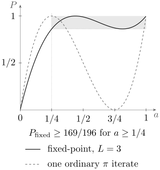
The fixed-point curve stays above $169/196$ for every $a\ge1/4$, despite small ripples. This compares response shapes, not equal Boolean-query costs: a standard sign change uses one Boolean call, while the displayed adjustable phase uses two. Both require forward and inverse preparations.

Approximate reflections and accumulated error

Approximate implementations require a separate error budget. Let $|\psi\rangle$ and $|\widetilde\psi\rangle$ be normalized, and let $\widetilde Q$ be unitary or, more generally, a contraction. Suppose

$$\|\widetilde Q-Q\|\le\eta$$

and

$$\||\widetilde\psi\rangle-|\psi\rangle\| \le \eta_0.$$

A telescoping sum and contractivity give

$$\| \widetilde Q^r|\widetilde\psi\rangle - Q^r|\psi\rangle \| \le \eta_0+r\eta.$$

For a unitary implementation these are normalized state vectors. For a contraction, the approximate vector can be subnormalized: its squared projection norm is a joint success probability before conditioning on the contraction having occurred. In either interpretation, the difference of squared projection norms is at most $2(\eta_0+r\eta)$. A sufficient allocation for overall state error of order $\epsilon$ is therefore $\eta=O(\epsilon/r)$ after budgeting preparation error. This worst-case coherent bound does not model stochastic hardware noise or prove fault-tolerant feasibility.

Operation counts and specialist variants

For $r$ ordinary iterates following one preparation, the exact component counts are

$$N_{\mathcal A}=r+1,\quad N_{\mathcal A^\dagger}=r, \qquad N_{S_G}=N_{S_0}=r.$$

Add measurement, verification and repetitions separately. Gates for preparation, inverse subroutines, controlled phases, workspace restoration and error correction determine the implementation cost. A reflection call and an elementary gate are different units.

The $1/\sqrt a$ scaling is worst-case optimal for fixed nontrivial target success in the generic black-box setting. Uniform preparation with one marked basis state has $a=1/N$; a universally faster amplifier would violate the unstructured-search lower bound. This does not imply every particular preparation is hard.

Boosting a reversible heuristic or heralded quantum preparation can be useful even when no general application speedup follows. Two further variants have additional assumptions: oblivious amplification uses block structure to act uniformly on unknown system inputs, while variable-time amplification uses coherent branches with different stopping times. See block encodings and QSVT and Hamiltonian simulation for the block-structured case, and Ambainis for the variable-time construction.

Two finite examples

A nonuniform preparation

In the ordered effective basis $\{|G\rangle,|B\rangle\}$, take

$$|\psi\rangle = \frac35|G\rangle + \frac45|B\rangle, \qquad a=\frac9{25},$$

so $\sin\theta=3/5$ and $\cos\theta=4/5$. The ideal iterate is

$$Q = \frac1{25} \begin{pmatrix} 7&24\\ -24&7 \end{pmatrix}.$$

Its columns are orthonormal, its determinant is one, and exact multiplication gives

$$Q|\psi\rangle = \frac{117}{125}|G\rangle - \frac{44}{125}|B\rangle.$$

Thus

$$p_1 = \frac{13689}{15625} = 0.876096.$$

A second iterate gives

$$Q^2|\psi\rangle = -\frac{237}{3125}|G\rangle - \frac{3116}{3125}|B\rangle,$$

and hence

$$p_2 = \frac{56169}{9765625} = 0.0057517056.$$

The norm identities $117^2+44^2=125^2$ and $237^2+3116^2=3125^2$ check both states. The second step has nearly erased the good component. A one-step run uses two forward preparations and one inverse; a two-step run uses three and two. These effective coefficients can multiply arbitrary normalized internal good and bad states, not only uniform search states.

Averaging an unknown-success window

Now take an unknown-success instance whose actual value is

$$a=\frac1{16},$$

and choose $R$ uniformly from $\{0,1,2,3\}$. The exact ordinary-iterate probabilities are

Iterations $r$	Success probability $p_r$
0	$1/16$
1	$121/256$
2	$3721/4096$
3	$63001/65536$

Putting the probabilities over a common denominator gives

$$\mathbb E[p_R] = \frac14 \left( \frac1{16} + \frac{121}{256} + \frac{3721}{4096} + \frac{63001}{65536} \right) = \frac{157609}{262144}.$$

Therefore

$$\mathbb E[p_R] = 0.601230621337890625.$$

The mean operation counts are $5/2$ forward preparations and $3/2$ inverses, plus $3/2$ calls to each reflection and one final test. This one window illustrates the averaging mechanism; it does not establish the full expected-cost theorem by itself.

Exercises

1. Normalize the good–bad decomposition

Let $|\psi\rangle$ be normalized and $a=\langle\psi|\Pi_G|\psi\rangle$. For $0<a<1$, prove that the definitions of $|G\rangle$ and $|B\rangle$ give an orthonormal pair and reconstruct $|\psi\rangle$. Then explain the $a=0$ and $a=1$ branches without dividing by zero.

Solution

Because $\Pi_G$ is an orthogonal projector,

$$\|\Pi_G|\psi\rangle\|^2 = \langle\psi|\Pi_G^2|\psi\rangle = a.$$

Similarly,

$$\|(I-\Pi_G)|\psi\rangle\|^2 = \langle\psi|(I-\Pi_G)|\psi\rangle = 1-a.$$

Thus the stated denominators normalize the two vectors. Their inner product is

$$\langle G|B\rangle = \frac{ \langle\psi|\Pi_G(I-\Pi_G)|\psi\rangle }{\sqrt{a(1-a)}} = 0.$$

Adding the two projected components gives

$$\sqrt a|G\rangle + \sqrt{1-a}|B\rangle = \Pi_G|\psi\rangle + (I-\Pi_G)|\psi\rangle = |\psi\rangle.$$

With $a=\sin^2\theta$ and $0<\theta<\pi/2$, the positive square roots are $\sin\theta$ and $\cos\theta$. If $a=0$, the good projection is the zero vector and no normalized $|G\rangle$ is defined or needed; the state is entirely bad. If $a=1$, the bad projection vanishes and the state is already entirely good.

2. Derive the reflection rotation and eigenphases

First use the Mathematical Projectors algebra to prove that $I-2P$ is a self-adjoint unitary for every orthogonal projector $P$. Then derive the two matrices defining $Q$, prove invariance of the good–bad plane, and find the eigenvalues of $Q$.

Solution

For $P=P^\dagger=P^2$,

$$(I-2P)^\dagger = I-2P,$$

and

$$(I-2P)^2 = I-4P+4P^2 = I.$$

The operator is therefore self-adjoint and its own inverse, hence unitary. Taking $P=\Pi_G$ gives

$$S_G = \begin{pmatrix} -1&0\\ 0&1 \end{pmatrix}$$

in the good–bad basis. Since $|\psi\rangle=(\sin\theta,\cos\theta)^{\mathsf T}$,

$$2|\psi\rangle\langle\psi|-I = \begin{pmatrix} 2\sin^2\theta-1&2\sin\theta\cos\theta\\ 2\sin\theta\cos\theta&2\cos^2\theta-1 \end{pmatrix}$$ $$= \begin{pmatrix} -\cos2\theta&\sin2\theta\\ \sin2\theta&\cos2\theta \end{pmatrix}.$$

Both matrices map the span of $|G\rangle$ and $|B\rangle$ to itself. Their product is

$$Q = \begin{pmatrix} \cos2\theta&\sin2\theta\\ -\sin2\theta&\cos2\theta \end{pmatrix}.$$

Its characteristic polynomial is

$$\lambda^2 - 2\cos2\theta\,\lambda + 1,$$

whose roots are $e^{\pm2i\theta}$. Multiplying the matrix by $(\sin\phi,\cos\phi)^{\mathsf T}$ gives $(\sin(\phi+2\theta),\cos(\phi+2\theta))^{\mathsf T}$, proving the stated rotation law.

3. Reproduce the rational nonuniform example

For $|\psi\rangle=(3|G\rangle+4|B\rangle)/5$, reproduce $Q|\psi\rangle$, $Q^2|\psi\rangle$, both exact success probabilities, the norm checks, and the operation counts for one and two iterates.

Solution

Here

$$\cos2\theta = \frac{16-9}{25} = \frac7{25}, \qquad \sin2\theta = 2\frac35\frac45 = \frac{24}{25}.$$

Therefore

$$Q \begin{pmatrix} 3/5\\ 4/5 \end{pmatrix} = \frac1{125} \begin{pmatrix} 7\cdot3+24\cdot4\\ -24\cdot3+7\cdot4 \end{pmatrix} = \frac1{125} \begin{pmatrix} 117\\ -44 \end{pmatrix}.$$

Applying $Q$ again gives

$$\frac1{3125} \begin{pmatrix} 7\cdot117-24\cdot44\\ -24\cdot117-7\cdot44 \end{pmatrix} = \frac1{3125} \begin{pmatrix} -237\\ -3116 \end{pmatrix}.$$

Hence

$$p_1 = \frac{117^2}{125^2} = \frac{13689}{15625},$$ $$p_2 = \frac{237^2}{3125^2} = \frac{56169}{9765625}.$$

The identities $117^2+44^2=125^2$ and $237^2+3116^2=3125^2$ verify normalization. For $r=1$, the tuple

$$(N_{\mathcal A},N_{\mathcal A^\dagger},N_{S_G},N_{S_0}) = (2,1,1,1)$$

is followed by one measurement. For $r=2$, it is $(3,2,2,2)$. Candidate verification, if required, is additional.

4. Prove the known-success stopping guarantee

Let $m=\lfloor\pi/(4\theta)\rfloor$. Prove $p_m\ge\max\{a,1-a\}$, show the resulting square-root scaling, and explain why certainty needs attenuation or a phase-adjusted final iterate.

Solution

For $0<a\le1/2$, one has $0<\theta\le\pi/4$. From

$$m \le \frac{\pi}{4\theta} < m+1$$

we obtain

$$-\theta \le \frac\pi2-(2m+1)\theta < \theta.$$

Writing the difference as $d$ gives

$$p_m = \sin^2\!\left(\frac\pi2-d\right) = \cos^2d \ge \cos^2\theta = 1-a.$$

For $a>1/2$, $\theta>\pi/4$, so $m=0$ and $p_m=a$. Thus the two cases give $p_m\ge\max\{a,1-a\}$. Since $\theta=\arcsin\sqrt a\ge\sqrt a$,

$$m \le \frac\pi{4\sqrt a}.$$

Ordinary iterates sample only angles $(2m+1)\theta$, which need not equal $\pi/2$ for an integer $m$. Attenuation changes the initial angle to one that lands exactly after an integer number of ordinary steps. A phase-adjusted terminal step instead changes the last rotation. Both require additional known-$a$ operations beyond the ordinary reflection interface.

5. Average an unknown-success window

For actual $a=1/16$, choose $R$ uniformly from $\{0,1,2,3\}$. Reproduce the four probabilities and their mean. Explain why candidate verification and the $a=0$ stopping behavior cannot be omitted from a full QSearch claim.

Solution

Let $s=\sin\theta=1/4$. Multiple-angle identities give

$$\sin3\theta = s(3-4s^2) = \frac{11}{16},$$ $$\sin5\theta = s(5-20s^2+16s^4) = \frac{61}{64},$$ $$\sin7\theta = s(7-56s^2+112s^4-64s^6) = \frac{251}{256}.$$

Squaring these amplitudes together with $\sin\theta=1/4$ gives

$$(p_0,p_1,p_2,p_3) = \left( \frac1{16}, \frac{121}{256}, \frac{3721}{4096}, \frac{63001}{65536} \right).$$

Over the common denominator $65536$, their numerator sum is $157609$, so

$$\mathbb E[p_R] = \frac{157609}{4\cdot65536} = \frac{157609}{262144}.$$

The mean forward count is $(1+2+3+4)/4=5/2$, and the mean inverse and each reflection count are $(0+1+2+3)/4=3/2$. Measurement alone can return an invalid candidate, so a verifier decides whether to stop. When $a=0$, every attempt fails; an uncapped exact procedure runs forever. A bounded decision claim therefore needs a positive-success promise or an explicit cutoff and error guarantee.

6. Check generalized and fixed-point phases

Use Høyer’s matching condition at $a=1/4$ and $\phi=\pi/2$. Then evaluate the Yoder–Low–Chuang threshold for $L=3$, $\delta=3\sqrt3/14$, and $a_0=1/4$.

Solution

The phase condition gives

$$\tan\frac\varphi2 = (1-2a)\tan\frac\phi2 = \frac12.$$

Therefore

$$\varphi = 2\arctan\frac12,$$

which is not $\phi=\pi/2$. Equal arbitrary phases would fail this matching test.

For the fixed-point values,

$$T_3\!\left(\frac2{\sqrt3}\right) = 4\left(\frac2{\sqrt3}\right)^3 - 3\left(\frac2{\sqrt3}\right) = \frac{14}{3\sqrt3} = \frac1\delta.$$

On the $x\ge1$ branch,

$$T_{1/3}(1/\delta) = \frac2{\sqrt3}.$$

Hence

$$w(3,\delta) = 1-\left(\frac2{\sqrt3}\right)^{-2} = \frac14.$$

At $a=a_0=1/4$, the argument of $T_3$ is one, so

$$P_3 = 1-\delta^2T_3(1)^2 = 1-\frac{27}{196} = \frac{169}{196}.$$

This is a uniform lower-bound guarantee with failure at most $27/196$, not exact success or monotonic improvement at every intermediate step. In the paper’s convention, $L=3$ uses $L-1=2$ Boolean target- oracle calls.

7. Budget approximate iterates

Assume normalized $|\psi\rangle$ and $|\widetilde\psi\rangle$, unitary $Q$, contractive $\widetilde Q$, $\|\widetilde Q-Q\|\le\eta$, and $\||\widetilde\psi\rangle-|\psi\rangle\|\le\eta_0$. Prove the linear telescoping bound and translate a target final state error $\epsilon$ into a sufficient per-iterate precision.

Solution

Add and subtract $\widetilde Q^r|\psi\rangle$. The preparation term satisfies

$$\| \widetilde Q^r(|\widetilde\psi\rangle-|\psi\rangle) \| \le \eta_0$$

by contractivity. For the iterate term, use

$$\widetilde Q^r-Q^r = \sum_{j=0}^{r-1} \widetilde Q^{r-1-j} (\widetilde Q-Q) Q^j.$$

Every summand has operator norm at most $\eta$, so

$$\| \widetilde Q^r|\widetilde\psi\rangle - Q^r|\psi\rangle \| \le \eta_0+r\eta.$$

If $\eta_0\le\epsilon/2$, choosing

$$\eta \le \frac{\epsilon}{2r}$$

is sufficient for final state error at most $\epsilon$. The difference between final squared projection norms is at most twice the vector distance. If the approximation is a contraction, this compares subnormalized branch probabilities; renormalizing a rare successful branch requires an additional bound on its probability. The bound still does not price synthesis, inverse circuits, ancillas, logical failure, error-correction cycles, routing, calibration, or physical time; those remain separate implementation costs.

8. Attenuate success to obtain an exact final state

For the nonuniform example with $a=9/25$, prepare an extra ancilla as $5|1\rangle/6+\sqrt{11}|0\rangle/6$ and declare success only when the original state is good and the ancilla is one. Find the joint initial success and the number of ordinary amplification iterations needed for exact success. What happens to the conditional state in the original good subspace?

Solution

The ancilla is normalized because $25/36+11/36=1$. The joint probability is

$$\bar a=\frac9{25}\frac{25}{36}=\frac14, \qquad \bar\theta=\frac\pi6.$$

One iterate therefore reaches angle $3\bar\theta=\pi/2$ and succeeds exactly. The new reflection about the prepared state uses the enlarged preparation and its inverse; simply appending the ancilla while retaining the old reflection would be a different algorithm. The joint good direction is $|G\rangle|1\rangle$, so the original normalized good component is preserved. Implementing the ancilla rotation exactly is an idealized gate assumption; approximate synthesis gives a corresponding error.

References

• A. Ambainis, “Variable Time Amplitude Amplification and a Faster Quantum Algorithm for Solving Systems of Linear Equations,” 29th International Symposium on Theoretical Aspects of Computer Science, LIPIcs 14, 636–647 (2012), doi:10.4230/LIPIcs.STACS.2012.636.
• D. W. Berry, A. M. Childs, R. Cleve, R. Kothari, and R. D. Somma, “Simulating Hamiltonian Dynamics with a Truncated Taylor Series,” Physical Review Letters 114, 090502 (2015), doi:10.1103/PhysRevLett.114.090502.
• M. Boyer, G. Brassard, P. Høyer, and A. Tapp, “Tight Bounds on Quantum Searching,” Fortschritte der Physik 46, 493–505 (1998), arXiv:quant-ph/9605034.
• G. Brassard, P. Høyer, M. Mosca, and A. Tapp, “Quantum Amplitude Amplification and Estimation,” Contemporary Mathematics 305, 53–74 (2002), doi:10.1090/conm/305/05215.
• L. K. Grover, “A Fast Quantum Mechanical Algorithm for Database Search,” in Proceedings of the 28th Annual ACM Symposium on Theory of Computing, 212–219 (1996), doi:10.1145/237814.237866.
• L. K. Grover, “Fixed-Point Quantum Search,” Physical Review Letters 95, 150501 (2005), doi:10.1103/PhysRevLett.95.150501.
• P. Høyer, “On Arbitrary Phases in Quantum Amplitude Amplification,” Physical Review A 62, 052304 (2000), doi:10.1103/PhysRevA.62.052304.
• M. A. Nielsen and I. L. Chuang, Quantum Computation and Quantum Information, 10th Anniversary Edition, Cambridge University Press (2010), doi:10.1017/CBO9780511976667.
• T. J. Yoder, G. H. Low, and I. L. Chuang, “Fixed-Point Quantum Search with an Optimal Number of Queries,” Physical Review Letters 113, 210501 (2014), doi:10.1103/PhysRevLett.113.210501.
• C. Zalka, “Grover’s Quantum Searching Algorithm Is Optimal,” Physical Review A 60, 2746–2751 (1999), doi:10.1103/PhysRevA.60.2746.