Quantum Phase Estimation

Quantum phase estimation (QPE) measures the phase of a unitary eigenvalue. If

$$U\lvert u\rangle=e^{2\pi i\phi}\lvert u\rangle, \qquad 0\leq\phi<1,$$

controlled powers of $U$ and an inverse Fourier transform produce an estimate of $\phi$. An exactly representable phase is recovered with certainty by the ideal circuit; otherwise the output has a calculable distribution of nearby values and tails. For a general target state, QPE also partially measures which eigenspace the target occupies.

This connects interference to spectroscopy, order finding and amplitude estimation. The essential resources are a suitable target preparation and coherent controlled powers, whose implementation can cost much more than the short binary answer suggests.

Helpful background. Phase kickback explains how a target eigenphase becomes a control’s relative phase; the quantum Fourier transform supplies the decoder and its bit-order convention.

Eigenphases and controlled evolution

An overall phase multiplying an isolated state is unobservable. A controlled operation makes it observable relative to the branch on which nothing happens:

$$\frac{\lvert0\rangle+\lvert1\rangle}{\sqrt2}\lvert u\rangle \longmapsto \frac{\lvert0\rangle+e^{2\pi i k\phi}\lvert1\rangle}{\sqrt2} \lvert u\rangle.$$

Here the control applies $U^k$ on its $\lvert1\rangle$ branch. The target remains in $\lvert u\rangle$, while interference on the control can reveal $k\phi$ modulo one. Increasing $k$ increases sensitivity but also creates more phase ambiguity; several powers resolve that ambiguity together.

An available implementation of $U$ does not automatically provide controlled-$U$, particularly for an unknown black box. A known circuit can be controlled gate by gate, with additional cost. Moreover, $U$ and $e^{i\alpha}U$ induce the same unconditional target channel but different controlled operations: $e^{i\alpha}$ becomes a relative control phase. A physical phase reference and the controlled implementation therefore belong to the problem specification.

The ideal analysis below assumes exact controlled powers and an exact inverse QFT. Implementation errors and imperfect target preparation are considered after the probability law.

From powered unitaries to a binary estimate

Let $L=2^m$ and write the control-register basis in most-significant-bit-first order,

$$\lvert k\rangle=\lvert k_{m-1}\cdots k_0\rangle, \qquad k=\sum_{j=0}^{m-1}2^j k_j.$$

Hadamards prepare $L^{-1/2}\sum_k\lvert k\rangle$. Control $k_j$ then applies $U^{2^j}$. On branch $k$, these powers multiply to $U^k$, giving

$$\begin{aligned} \frac1{\sqrt L}\sum_{k=0}^{L-1}\lvert k\rangle U^k\lvert u\rangle &=\frac1{\sqrt L}\sum_{k=0}^{L-1} e^{2\pi i k\phi}\lvert k\rangle\lvert u\rangle. \end{aligned}$$

The controls now form a phase-gradient state: neighboring basis amplitudes differ by $e^{2\pi i\phi}$. The target factors out because it is an eigenstate.

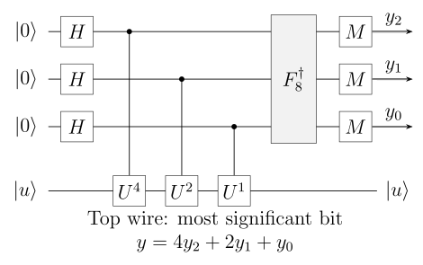
The top control is the most significant bit, so it controls $U^4$. The block $F_8^\dagger$ includes the bit ordering in the displayed Fourier definition; the measured integer is $y=4y_2+2y_1+y_0$. For an eigenstate the target is unchanged.

Use the positive-sign Fourier convention

$$F_L\lvert a\rangle=\frac1{\sqrt L} \sum_{k=0}^{L-1}e^{2\pi i ka/L}\lvert k\rangle.$$

If $\phi=a/L$, the control state is exactly $F_L\lvert a\rangle$. Applying $F_L^\dagger$ returns $\lvert a\rangle$ and measurement gives $a$ with certainty. For example, $\phi=3/8=0.011_2$ produces $\lvert011\rangle$. This non-palindromic example also detects an omitted bit reversal: $110$ would mean six, not three, unless the readout is explicitly reversed.

An exact $m$-qubit QFT has an $O(m^2)$ elementary decomposition. Approximate QFT circuits omit sufficiently small rotations, introducing a separate error. See the QFT derivation for the gates and swaps. One measurement still returns one integer, not an entire list of eigenvalues.

Finite-resolution phase probabilities

For an arbitrary phase, the amplitude of outcome $y$ after the inverse QFT is

$$a_y(\phi)=\frac1L\sum_{k=0}^{L-1} e^{2\pi i k(\phi-y/L)}.$$

Phases live on a circle. Define

$$\begin{aligned} d_{\mathbb T}(x,z)&=\min_{\ell\in\mathbb Z}|x-z-\ell|,\\ \delta_y&=\phi-y/L-\ell_y\in[-1/2,1/2). \end{aligned}$$

Subtracting the integer $\ell_y$ leaves the exponential sum unchanged. Summing its geometric progression gives

$$\begin{aligned} a_y(\phi)&=e^{\pi i(L-1)\delta_y} \frac{\sin(\pi L\delta_y)}{L\sin(\pi\delta_y)},\\ \Pr(Y=y)&=\frac{\sin^2(\pi L\delta_y)} {L^2\sin^2(\pi\delta_y)}. \end{aligned}$$

At $\delta_y=0$ take the continuous value $a_y=1$. The tails are part of the ideal measurement distribution. In particular, a phase near one can yield $y=0$ with high probability: that is a nearby estimate on the circle.

For $\phi=0.3$ and $L=8$, direct substitution gives

$$\Pr(Y=2)\approx0.578,\qquad \Pr(Y=3)\approx0.259.$$

These adjacent bins carry about $0.837$ of the probability. A single result $2/8$ is an estimate with error $0.05$, not an assertion that the unknown phase equals $0.25$.

Nearest bin and confidence

Choose a nearest grid point $y_\star/L$ on the circle, including either choice at a tie. Its distance is at most $1/(2L)$, and elementary sine bounds yield

$$\Pr(Y=y_\star)\geq\frac4{\pi^2}\approx0.405.$$

This is a guarantee for one particular bin, and is below one half. It alone does not justify majority voting on that bin. Confidence can instead be increased by accepting a specified neighborhood and using additional phase qubits, or by a repetition scheme with a proved success event. Arithmetic averages or medians of representatives in $[0,1)$ require particular care at the zero/one seam.

Extra phase qubits and what to report

State accuracy as an inequality. For $n\geq1$ and $0<\epsilon<1$, a sufficient choice is

$$\begin{aligned} m&=n+s,\\ s&=\left\lceil\log_2\left(2+\frac1{2\epsilon}\right)\right\rceil. \end{aligned}$$

Then the unrounded estimate $\widehat\phi=Y/2^m$ obeys

$$\Pr\!\left[d_{\mathbb T}(\widehat\phi,\phi)>2^{-n}\right] \leq\epsilon.$$

Here is a direct, conservative tail argument. Put $x=Ld_{\mathbb T}(y/L,\phi)$. For $x>0$, the denominator bound $|\sin(\pi\delta_y)|\geq2|\delta_y|$ gives $\Pr(Y=y)\leq1/(4x^2)$. At most two outcomes have distance $x$ in each interval $[r,r+1)$. The failure event has $x>2^s$, so

$$\Pr(\text{failure}) \leq\frac12\sum_{r=2^s}^{\infty}\frac1{r^2} \leq\frac1{2(2^s-1)} \leq\epsilon.$$

The chosen number of qubits is sufficient, not optimal. It guarantees proximity, not recovery of a uniquely defined first $n$ binary digits for phases arbitrarily close to a binary boundary.

Rounding $\widehat\phi$ to the nearest $n$-bit grid point adds at most $2^{-(n+1)}$ of circular error; discarding digits can add almost $2^{-n}$. If the final answer must be rounded to $n$ bits while retaining error at most $2^{-n}$, run the same bound with target raw error $2^{-(n+1)}$ first. One extra phase qubit then leaves room for the rounding error.

Finite-resolution measurement of a general target

Let the distinct unitary eigenvalues have spectral projectors $P_\lambda$:

$$U=\sum_\lambda e^{2\pi i\phi_\lambda}P_\lambda.$$

Reading the control outcome $y$ applies the target Kraus operator

$$K_y=\frac1L\sum_{k=0}^{L-1}e^{-2\pi i ky/L}U^k =\sum_\lambda a_y(\phi_\lambda)P_\lambda.$$

Thus, for any initial density operator $\rho$,

$$\begin{aligned} p_y&=\sum_\lambda |a_y(\phi_\lambda)|^2 \operatorname{Tr}(P_\lambda\rho),\\ \rho_y&=K_y\rho K_y^\dagger/p_y\quad(p_y>0). \end{aligned}$$

The probabilities are a weighted mixture of phase distributions because different eigenspaces are orthogonal. The conditional state need not be an eigenstate: several eigenspaces can contribute coherently to the same bin. Within a degenerate eigenspace, $K_y$ is a scalar, so it does not resolve or dephase the vectors inside that eigenspace.

For a concrete example, take $L=4$, two orthogonal eigenvectors with phases $0$ and $1/6$, and input $(\lvert u_0\rangle+\lvert u_1\rangle)/\sqrt2$. Outcome zero has amplitudes

$$a_0(0)=1,\qquad a_0(1/6)=\frac{i\sqrt3}{4}.$$

It therefore occurs with probability $19/32$ and leaves

$$\lvert\psi_0\rangle =\frac{4\lvert u_0\rangle+i\sqrt3\lvert u_1\rangle}{\sqrt{19}}.$$

This finite-resolution filter preserves a superposition. Exact projective measurement is obtained when all relevant distinct phases lie on distinct grid points; well-separated peaks approximate that behavior.

No amplitude is created in an eigenspace absent from the input. However, Fourier tails can produce numerical estimates near an eigenphase that is absent. Those are different claims. Likewise, QPE does not favor low energy by itself: a well-resolved, identifiable eigenspace of initial weight $w$ requires order $1/w$ fresh attempts to see once on average. Finite-resolution false positives and preparation errors must also be included when accepting a result as a particular energy.

Discarding the phase register

Ignoring the readout averages the conditional states with their probabilities. Substituting $K_y$ and using discrete Fourier orthogonality, $\sum_{y=0}^{L-1}e^{-2\pi i(k-k')y/L}=L\delta_{kk'}$, gives

$$\mathcal E_L(\rho)=\sum_y p_y\rho_y =\sum_y K_y\rho K_y^\dagger =\frac1L\sum_{k=0}^{L-1}U^k\rho U^{-k}.$$

The same channel results if the control register is simply traced out, even before the inverse QFT. A unitary acting only on that discarded register cannot change the target’s reduced state. This is an average over coherent evolutions, not a prescription to replace every run by a particular eigenstate.

In the spectral decomposition, each coherence block is multiplied by

$$P_\lambda\mathcal E_L(\rho)P_\mu =\left[\frac1L\sum_{k=0}^{L-1} e^{2\pi i k(\phi_\lambda-\phi_\mu)}\right] P_\lambda\rho P_\mu.$$

Consequently, eigenspace populations and all coherence within a degenerate eigenspace are preserved. Distinct phases on the $L$-point grid have zero multiplier, recovering the nonselective projective measurement $\sum_\lambda P_\lambda\rho P_\lambda$. At finite resolution, off-grid coherences can survive, as the example above illustrates.

Discarding the phase register therefore generally changes the target, even when no result is used. To restore an arbitrary input coherently, retain the register and reverse the entire ideal QPE circuit before measurement or other loss of coherence. Reversing only the inverse QFT leaves the controlled-power entanglement in place.

Precision, evolution time and implementation error

There are $m$ controlled-power blocks, but their cost depends on the available operations:

Available operation	Implementing $U^{2^j}$	Total cost of the powers
Supplied powered-unitary primitive	One call to the specified power	$m$ calls in this stronger access model
Repeated controlled-$U$	$2^j$ base calls	$2^m-1$ base calls
Controlled Hamiltonian simulation	Evolution for time $2^j\tau$	Simulated durations sum to $(2^m-1)\tau$

Structured arithmetic can implement powers efficiently without literal repetition, as in Shor’s algorithm. For energy estimation with $U=e^{-iH\tau/\hbar}$, the total interrogation time in the standard sequential circuit is

$$T_{\rm tot}=(2^m-1)\tau.$$

The longest individual block lasts $2^{m-1}\tau$; the target remains coherent across all blocks and the decoder. At fixed confidence, the bin scale gives an energy resolution of order $\hbar/T_{\rm tot}$. More confidence or a small initial overlap increases the total experimental cost. Merely counting output bits or controlled-power boxes hides these costs.

To separate implementation from ideal statistical error, suppose the target preparation has trace distance at most $\eta_{\rm prep}$ from the specified input. If implemented controlled blocks differ from their ideal unitaries in operator norm by at most $\eta_j$, and the inverse QFT differs by at most $\eta_F$, telescoping the circuit and using measurement contractivity bounds the change in any output-event probability by

$$\eta_{\rm prep}+\sum_j\eta_j+\eta_F.$$

This bound applies to unitary implementation errors; general noise can instead be bounded using channel distances. Long powers are often harder because simulation and calibration errors accumulate with duration. An operator-norm error does not receive an additional weight merely because its block has the largest power. For repeated base gates each of error at most $\eta$, a conservative total contribution is $(2^m-1)\eta$.

Energy estimation without a phase ambiguity

For $H\lvert E\rangle=E\lvert E\rangle$, the shifted unitary

$$U=e^{-i(H-E_{\rm ref}I)\tau/\hbar}$$

has eigenphase

$$\phi_E=\frac{(E_{\rm ref}-E)\tau}{2\pi\hbar}\pmod1.$$

The minus sign follows from the time-evolution operator. The offset is a genuine control phase and must be implemented consistently. An energy interval of width $W=E_{\max}-E_{\min}>0$ is mapped injectively into the phase circle if $W\tau<2\pi\hbar$.

Injectivity of the exact mapping alone does not make naive finite-precision decoding safe. Taking $E_{\rm ref}=E_{\max}$ puts the upper endpoint at phase zero, so a nearby estimate just below one must be unwrapped before converting it to an energy.

A convenient alternative puts the entire promised interval away from that seam:

$$E_{\rm ref}=E_{\max}+\frac W2,\qquad \tau=\frac{\pi\hbar}{W}.$$

Then $\phi_E\in[1/4,3/4]$. If the circular phase error is strictly less than $1/4$, the reported representative in $[0,1)$ has the same ordinary absolute error, and

$$\widehat E=E_{\rm ref}-2W\widehat\phi, \qquad |\widehat E-E|=2W|\widehat\phi-\phi_E|.$$

For example, a promised range $[2,6]$ in a chosen energy unit gives $W=4$, $E_{\rm ref}=8$ and $\phi_E=(8-E)/8$. Energy $E=3$ has phase $5/8$; phase error at most $1/128$ means energy error at most $1/16$ in that unit. If $W=0$, the promised energy is already known and this construction is unnecessary.

Abrams and Lloyd developed the eigenvalue application; molecular examples and resource studies include Aspuru-Guzik and collaborators and Reiher and collaborators. A useful calculation must include preparation overlap and controlled-evolution error, not only phase bins. Trotter–Suzuki methods treats one implementation and its energy bias; digital quantum simulation places it among other methods.

Semiclassical and iterative measurements

The Griffiths–Niu construction replaces a Fourier transform immediately followed by computational-basis measurement with sequential one-qubit measurements and classical phase corrections. It preserves those output statistics; it does not implement a coherent Fourier transform for use by a later quantum subroutine. Reordering the controlled powers appropriately also allows the phase register to be replaced by a reused ancilla.

In an iterative protocol, each round applies a selected controlled power and a correction determined by earlier outcomes. Width decreases, but rounds become sequential and accurate measurement, reset and feedforward matter. The largest required power remains. Dobšíček and collaborators give a concrete single-ancilla implementation.

For an eigenstate, the target can be retained or the same eigenstate can be prepared again. For an unknown superposition, retaining the target preserves the correlations that make successive bits refer to a common phase. Preparing a fresh superposition independently for every bit generally samples different latent eigenphases and need not reproduce standard QPE. Repeated statistical experiments on such inputs require an explicit mixture-estimation analysis.

Kitaev’s approach instead estimates sine and cosine quadratures of $e^{2\pi i k\phi}$ for selected powers, then combines their modular information classically. One experiment with control correction $\operatorname{diag}(1,e^{-i\beta})$ followed by a Hadamard gives

$$\Pr(0\mid k,\beta) =\frac{1+\cos(2\pi k\phi-\beta)}2.$$

Choosing $\beta=0$ or $\pi/2$ reveals the two quadratures through repeated samples. This trades a coherent multi-qubit decoder for statistical inference; it does not make long controlled evolution or state preparation free.

Exercises

1. Exact phase and bit reversal

For $\phi=3/8$ and three control qubits, find the state before and after $F_8^\dagger$. Why is this a better bit-order test than $\phi=5/8$?

Solution

The control state is $8^{-1/2}\sum_{k=0}^7 e^{2\pi i3k/8}\lvert k\rangle=F_8\lvert3\rangle$. The inverse produces $\lvert3\rangle=\lvert011\rangle$ with certainty. Reversing the readout gives $110$, which would be decoded as six without a reversal correction. The string $101$ for $5/8$ is a palindrome and would conceal this mistake.

2. Derive the phase-gradient state

Starting from $\lvert+\rangle^{\otimes m}\lvert u\rangle$, derive the phase-gradient state by considering one computational branch.

Solution

On $\lvert k_{m-1}\cdots k_0\rangle$, the target operation is

$$\prod_{j=0}^{m-1}U^{2^j k_j} =U^{\sum_j2^j k_j}=U^k.$$

It contributes $e^{2\pi i k\phi}$ and leaves the eigenstate unchanged. Summing all branches with their original amplitude $2^{-m/2}$ gives the stated phase gradient. The tensor order and integer weights must agree; reversing only the powers changes this state.

3. Nearest-bin probability and rounding

Prove the $4/\pi^2$ nearest-bin bound. If a raw estimate is within $2^{-(n+1)}$ of the phase on the circle, bound its error after rounding to the nearest $n$-bit phase.

Solution

For the nearest bin, $|\delta|\leq1/(2L)$. The inequalities $\sin x\geq2x/\pi$ for $0\leq x\leq\pi/2$ and $\sin x\leq x$ give

$$|\sin(\pi L\delta)|\geq2L|\delta|, \qquad L|\sin(\pi\delta)|\leq\pi L|\delta|.$$

Hence $|a_y|\geq2/\pi$, and squaring proves the claim. The value at zero follows by continuity. Rounding adds at most $2^{-(n+1)}$; the triangle inequality for circular distance gives final error at most $2^{-n}$. This is a proximity statement, not a guarantee of the same truncated binary digits as the exact phase.

4. Resolved and unresolved eigenspaces

Suppose the input is $\sqrt{0.7}\lvert u_1\rangle+e^{i\gamma}\sqrt{0.3}\lvert u_2\rangle$. Find the outcome probabilities and target states when the phases occupy distinct exact grid points. Then verify the $L=4$, phases $0,1/6$ example in the text and explain the difference. For that equal-weight input, find the target density matrix and purity when the readout is ignored. Does ignoring it restore the initial state?

Solution

For exact distinct bins, the final state is $\sqrt{0.7}\lvert y_1\rangle\lvert u_1\rangle+e^{i\gamma}\sqrt{0.3}\lvert y_2\rangle\lvert u_2\rangle$. Outcomes have probabilities $0.7$ and $0.3$ and leave the corresponding eigenstates. Orthogonality of the readouts removes $\gamma$ from these probabilities.

For the finite-resolution example,

$$a_0(1/6)=\frac{1+e^{i\pi/3}+e^{2i\pi/3}+e^{i\pi}}4 =\frac{i\sqrt3}4.$$

With equal input weights, $p_0=(1+3/16)/2=19/32$. Normalizing $(\lvert u_0\rangle+i\sqrt3\lvert u_1\rangle/4)/\sqrt2$ gives $(4\lvert u_0\rangle+i\sqrt3\lvert u_1\rangle)/\sqrt{19}$. The same readout now receives both eigenphase amplitudes, so the conditional target retains their coherence.

For the ignored readout, the $01$ coherence is multiplied by $a_0(-1/6)=-i\sqrt3/4$. In the ordered basis $(\lvert u_0\rangle,\lvert u_1\rangle)$,

$$\mathcal E_4(\rho)= \begin{pmatrix} 1/2&-i\sqrt3/8\\ i\sqrt3/8&1/2 \end{pmatrix},\qquad \operatorname{Tr}[\mathcal E_4(\rho)^2]=\frac{19}{32}.$$

The initial pure state’s off-diagonal entries were $1/2$. Its populations are unchanged, but its coherence and purity have decreased. The averaged state is neither the original state nor the fully dephased $I/2$. Coherently reversing QPE before reading or discarding its register would instead restore the original state.

5. Energy interval and the phase seam

For $U=e^{-i(H-E_{\max}I)\tau/\hbar}$, derive the no-aliasing condition on a promised interval of width $W$. Explain the possible decoding error near $E_{\max}$, and show how the interior-interval choice in the text avoids it on its success event.

Solution

The exact phase is $(E_{\max}-E)\tau/(2\pi\hbar)$. If $W\tau<2\pi\hbar$, it lies in one interval of width less than one and determines

$$E=E_{\max}-\frac{2\pi\hbar\phi_E}{\tau}.$$

But a true phase $\phi_E=\delta$ close to zero and an estimate $1-\delta$ have circular error $2\delta$, while naive subtraction uses an error near one. With $E_{\rm ref}=E_{\max}+W/2$ and $\tau=\pi\hbar/W$, the exact interval becomes $[1/4,3/4]$. A circular error strictly below $1/4$ cannot cross the seam, so ordinary energy decoding has error exactly $2W$ times the phase error.

6. Count the powers

If powers are implemented by repeated controlled-$U$, count the base calls. Compare three distinct resource counts for $m=3$ and base evolution duration $\tau$.

Solution

The count is $\sum_{j=0}^{m-1}2^j=2^m-1$, of order $1/\Delta\phi$ at fixed confidence. For $m=3$ there are three controlled-power blocks, seven base calls and maximum individual duration $4\tau$. Their sequential durations sum to $7\tau$, before decoding and other gates. Those counts describe different resources.

7. One-control quadratures

Apply $\operatorname{diag}(1,e^{-i\beta})$ and then a Hadamard to $(\lvert0\rangle+e^{2\pi i k\phi}\lvert1\rangle)/\sqrt2$. Find $\Pr(0)$ for $\beta=0$ and $\pi/2$.

Solution

The amplitude of zero is $[1+e^{i(2\pi k\phi-\beta)}]/2$. Its squared modulus is $[1+\cos(2\pi k\phi-\beta)]/2$. The two choices give

$$\Pr(0\mid\beta=0)=\frac{1+\cos(2\pi k\phi)}2, \qquad \Pr(0\mid\beta=\pi/2)=\frac{1+\sin(2\pi k\phi)}2.$$

Estimating both quadratures removes the cosine-only reflection ambiguity. Multiple powers and repeated samples are still needed to resolve the phase to a chosen accuracy with a stated confidence.

References

• D. S. Abrams and S. Lloyd, “Quantum algorithm providing exponential speed increase for finding eigenvalues and eigenvectors,” Physical Review Letters 83, 5162–5165, 1999, doi:10.1103/PhysRevLett.83.5162.
• A. Aspuru-Guzik, A. D. Dutoi, P. J. Love, and M. Head-Gordon, “Simulated quantum computation of molecular energies,” Science 309, 1704–1707, 2005, doi:10.1126/science.1113479.
• R. Cleve, A. Ekert, C. Macchiavello, and M. Mosca, “Quantum algorithms revisited,” Proceedings of the Royal Society A 454, 339–354, 1998, doi:10.1098/rspa.1998.0164.
• M. Dobšíček, G. Johansson, V. Shumeiko, and G. Wendin, “Arbitrary accuracy iterative quantum phase estimation algorithm using a single ancillary qubit: A two-qubit benchmark,” Physical Review A 76, 030306(R), 2007, doi:10.1103/PhysRevA.76.030306.
• R. B. Griffiths and C.-S. Niu, “Semiclassical Fourier transform for quantum computation,” Physical Review Letters 76, 3228–3231, 1996, doi:10.1103/PhysRevLett.76.3228.
• A. Yu. Kitaev, “Quantum measurements and the Abelian stabilizer problem,” 1995, arXiv:quant-ph/9511026.
• M. A. Nielsen and I. L. Chuang, Quantum Computation and Quantum Information, 10th anniversary ed., Cambridge University Press, 2010, doi:10.1017/CBO9780511976667.
• M. Reiher, N. Wiebe, K. M. Svore, D. Wecker, and M. Troyer, “Elucidating reaction mechanisms on quantum computers,” Proceedings of the National Academy of Sciences 114, 7555–7560, 2017, doi:10.1073/pnas.1619152114.
• P. W. Shor, “Polynomial-time algorithms for prime factorization and discrete logarithms on a quantum computer,” SIAM Journal on Computing 26, 1484–1509, 1997, doi:10.1137/S0097539795293172.