Quantum Algorithms for Chemistry and Materials

Quantum algorithms for chemistry and materials estimate properties of a specified Hamiltonian: an energy, a transition strength, a time correlation or a thermal average. Choosing an algorithm begins with that property. A method that estimates one eigenvalue does not by itself give a reaction barrier, an optical spectrum or a transport coefficient.

Two approximations must be kept distinct. A finite basis or active space changes the physical model being solved; a quantum solver approximates the answer within that model. An exact fermion-to-qubit transformation changes the representation without adding model error. Below, small Hamiltonians make these distinctions concrete, and connect them to state preparation, phase estimation, variational methods and measurement cost. McArdle and collaborators and Bauer and collaborators provide broader reviews McArdle et al. (2020), Bauer et al. (2020).

Helpful background. Many-particle Hamiltonians introduces occupation operators and particle-number sectors; Hamiltonian simulation explains controlled evolution and block encodings; algorithmic primitives distinguishes state preparation, queries and classical outputs.

Electronic Hamiltonians and the requested property

Fix nuclear positions and a finite orthonormal spin-orbital basis. In atomic units ($\hbar=1$), a common clamped-nuclei Hamiltonian is

$$H=E_{\rm nuc}+\sum_{pq}h_{pq}a_p^\dagger a_q +\frac14\sum_{pqrs}\langle pq\Vert rs\rangle a_p^\dagger a_q^\dagger a_s a_r.$$

The two-electron integrals here are antisymmetrized. An expression using unsymmetrized integrals instead has a factor $1/2$ with the corresponding index convention. Mixing these conventions gives a different operator. $E_{\rm nuc}$ is a scalar at the fixed geometry but changes along a reaction coordinate. The molecular Hamiltonian explains the physical approximations and integral definitions.

The basis size, geometry, charge and relevant symmetry sector determine the finite calculation. Orbital truncation, nuclear motion, relativistic effects and the environment can matter even when a solver returns many digits. For a true variational restriction of the same parent Hamiltonian, the restricted ground energy remains an upper bound to the parent ground energy. An independently fitted or approximate effective Hamiltonian need not have that ordering.

The output must also be specified. A reaction energy is a difference between geometries, so consistent approximations and possible cancellation matter. An optical transition needs a neutral excitation energy and a nonzero transition matrix element. For a finite system with well-defined particle sectors, the charge gap is instead

$$\Delta_{\rm c}=E_0(N+1)+E_0(N-1)-2E_0(N).$$

It differs from the neutral excitation $E_1(N)-E_0(N)$. Relating either to a measured bulk spectrum requires the appropriate finite-size treatment, selection rules and physical environment.

Lattice and periodic materials

A lattice model such as

$$H_{\rm Hub}=-t\sum_{\langle i,j\rangle,\sigma} (c_{i\sigma}^\dagger c_{j\sigma}+c_{j\sigma}^\dagger c_{i\sigma}) +U\sum_i n_{i\uparrow}n_{i\downarrow}$$

is a different starting point from a full electronic-structure calculation. Here each unordered bond appears once, with real hopping $t$. The graph, boundary conditions, filling and parameter values are part of the model. Such a model can test a physical mechanism without describing every property of a material.

Periodic electronic calculations additionally use a cell, momentum sampling and a one-particle basis. Plane waves make kinetic energy diagonal; a dual basis can simplify interactions. Bloch integrals can be complex and conserve crystal momentum modulo reciprocal-lattice vectors. These structures affect the simulation cost Babbush et al. (2018), Rubin et al. (2023). Cell-size and basis convergence remain separate from the accuracy of quantum time evolution.

Second quantization uses occupation registers for modes. First quantization uses particle registers, with antisymmetry imposed on the state. For $N$ particles and $M$ one-particle modes, the latter can reduce register width to a scale $N\log M$, but antisymmetrization, arithmetic and input preparation still cost operations. Su and collaborators develop a fault-tolerant first-quantized construction Su et al. (2021). The useful comparison is between complete implementations of the same finite problem, not qubit counts in isolation.

Exact fermion encodings

Order the spin orbitals as $0,1,\ldots,M-1$, and use $|n_0n_1\cdots n_{M-1}\rangle$ with qubit zero the leftmost factor. Jordan–Wigner gives

$$a_p=\left(\prod_{j<p}Z_j\right)\frac{X_p+iY_p}{2}, \qquad n_p=\frac{I-Z_p}{2}.$$

The parity string supplies the fermionic sign. Without it, operators on different qubits commute rather than anticommute. This is an exact mapping of the finite Fock space Jordan and Wigner (1928); the Jordan–Wigner derivation explains the algebra in detail.

Bravyi–Kitaev encodings store combinations of occupation and parity, with logarithmic support for elementary updates in the usual tree construction Bravyi and Kitaev (2002), Seeley et al. (2012). This can shorten operators but does not establish a universal advantage after term grouping, routing and state preparation. Both encodings must transform the Hamiltonian, prepared state and measured operators consistently.

Worked example: two modes, one exact operator

Consider

$$H=\epsilon_0n_0+\epsilon_1n_1 +t(a_0^\dagger a_1+a_1^\dagger a_0)+Un_0n_1,$$

with $\epsilon_0=-1$, $\epsilon_1=0.5$, $t=0.25$ and $U=0.75$. This toy hopping sign is explicitly positive $t$, unlike the Hubbard convention above. In the basis $|00\rangle,|01\rangle,|10\rangle,|11\rangle$,

$$H=\begin{pmatrix} 0&0&0&0\\ 0&0.5&0.25&0\\ 0&0.25&-1&0\\ 0&0&0&0.25 \end{pmatrix}.$$

The qubit form is

$$H={}-0.0625I+0.3125Z_0-0.4375Z_1 +0.1875Z_0Z_1+0.125(X_0X_1+Y_0Y_1).$$

Expanding $n_0n_1=(I-Z_0-Z_1+Z_0Z_1)/4$ produces the diagonal terms. The hopping term becomes $(X_0X_1+Y_0Y_1)/2$: it exchanges $|01\rangle$ and $|10\rangle$ while leaving vacuum and double occupation unchanged. The one-particle energies are

$$E_\pm=\frac{-0.5\pm\sqrt{2.5}}2.$$

The vacuum and two-particle energies are $0$ and $0.25$. Therefore the neutral gap within $N=1$ is $\sqrt{2.5}$, whereas the charge gap at $N=1$ is $0.75+\sqrt{2.5}$. They are distinct even in this four-dimensional example.

Active spaces and virtual excitations

Freezing core occupations and selecting active orbitals reduces the number of configurations. It also changes which fluctuations are represented. The frozen modes contribute scalar and one-body shifts, which must be kept. Consistent orbital choices along a geometry scan help avoid artificial jumps; enlarging the active space tests a different error from improving the solver.

Let $P$ project onto the retained configurations and $Q=I-P$. If $E-QHQ$ is invertible on the omitted subspace, eliminating $Q|\psi\rangle$ from the eigenvalue equation gives

$$H_{\rm eff}(E)=PHP+PHQ(E-QHQ)^{-1}QHP.$$

The second term describes virtual excursions into omitted configurations. It is energy dependent; replacing the full Hamiltonian by $PHP$ discards it. Perturbative downfolding approximates such effects under a separation of energy scales, whereas a fitted effective model uses additional physical input.

For the two-configuration matrix

$$H=\begin{pmatrix}0&g\\g&\Delta\end{pmatrix},\qquad\Delta>0,$$

retaining only the first configuration gives energy zero. The exact ground energy is instead

$$E_-=\frac{\Delta-\sqrt{\Delta^2+4g^2}}2 =-\frac{g^2}{\Delta}+O(g^4/\Delta^3).$$

The lowest-order correction is reliable for $|g|/\Delta\ll1$. At $g/\Delta=0.2$, the exact value is about $-0.038516\Delta$, while second order gives $-0.04\Delta$. An arbitrarily precise solver for the retained one-dimensional Hamiltonian still returns zero.

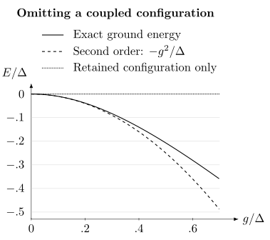
Omitted configurations shift the low energy through virtual transitions. The retained-only model gives zero at every coupling; the second-order correction follows the exact result only when $|g|/\Delta$ is small. Solver precision and active-space accuracy are separate questions.

Symmetry reduction and transition operators

Commuting $\mathbb Z_2$ Pauli symmetries can reduce qubit count after their eigenvalues are fixed. A suitable Clifford transformation isolates the symmetry labels so that redundant qubits can be removed Bravyi et al. (2017). Selecting the wrong sector removes the desired state; more precise diagonalization cannot recover it.

An operator used for a transition may change the sector. If $S^2=I$, $\Pi_s=(I+sS)/2$ and $\{O,S\}=0$, then $\Pi_s O\Pi_s=0$, although $\Pi_{-s}O\Pi_s$ can be nonzero. Its transition strength cannot be computed using only the matrix of $O$ inside one tapered sector. For example, a particle-creation operator changes fermion parity. Energy calculations and addition/removal spectra can therefore require different retained sectors.

Initial states and the probability of finding a level

A Slater determinant is inexpensive to prepare but may have poor overlap with a strongly correlated ground state. Multiconfigurational states, tensor-network states, variational preparations and adiabatic paths offer alternatives with their own classical and quantum costs. Fomichev and collaborators emphasize the prepared state’s full energy distribution, not just a circuit’s depth Fomichev et al. (2024).

For a target eigenspace with projector $\Pi_0$, define $p_0=\langle\phi|\Pi_0|\phi\rangle$. An ideal projective energy measurement hits that eigenspace with probability $p_0$. Independent preparations then give success probability $1-(1-p_0)^R$ after $R$ trials. For $0<p_0<1$,

$$R\ge\left\lceil\frac{\log\delta}{\log(1-p_0)}\right\rceil$$

suffices for failure probability at most $\delta$. The ideal target hit is impossible if $p_0=0$ and certain in one trial if $p_0=1$.

Finite-resolution phase estimation has another probability. If its conditional probability of returning an adequately accurate target energy is at least $q$, then $p_0q$ is a lower bound on the per-trial probability of that good event. Replacing $p_0$ by $p_0q$ gives a sufficient repetition count. Even $p_0=1$ does not guarantee an accurate estimate in one finite trial when $q<1$. Identifying a returned result as the ground level also requires controlling false assignments from other levels, using separation, filters or other information. Merely taking the smallest noisy output is not a reliable ground-energy bound.

A small energy variance does not certify ground-state overlap: an exact excited eigenstate has variance zero and $p_0=0$. Energy-based overlap bounds need a ground-energy lower bound and a gap estimate, as explained in VQE. For a spectrum rather than a single level, a state with several eigencomponents can be useful; a transition operator changes their weights.

Phase estimation: energy resolution and confidence

Use $U=\exp[-i(H-E_{\rm ref})\tau]$ and the convention $U|E_k\rangle=e^{2\pi i\phi_k}|E_k\rangle$. Then

$$\phi_k=-\frac{(E_k-E_{\rm ref})\tau}{2\pi}\pmod1.$$

The minus sign and the integer branch matter. Choose a promised energy interval strictly narrower than $2\pi/\tau$, or use a suitable half-open interval with specified endpoint conventions. Energies separated by $2\pi/\tau$ give identical phases. For a correctly unwrapped representative, $E_k=E_{\rm ref}-2\pi\phi_k/\tau$.

If $W=2\pi/\tau$ is the decoding period and an $m$-bit register is used, the grid spacing and total controlled evolution time of ordinary Fourier phase estimation are

$$\Delta E=\frac{W}{2^m},\qquad T_{\rm int}=\frac{2\pi}{W}(2^m-1).$$

Time here is in atomic units. This interaction time is not wall-clock runtime. More importantly, the grid spacing is not a deterministic error bound: a non-grid eigenphase has a distribution over outcomes with tails. Confidence needs extra phase bits or another specified estimation procedure. Independent runs on freshly prepared superpositions can sample different eigenvalues, so taking their median is not generally confidence amplification for one particular eigenvalue.

For example, $W=8$ hartree and $m=13$ give $\Delta E=0.0009765625$ hartree and $T_{\rm int}=(\pi/4)8191$. These numbers describe resolution and ideal interaction time; they do not alone guarantee millihartree accuracy with 99% probability. The full distribution and conditional output state are derived in quantum phase estimation. Aspuru-Guzik and collaborators developed an early electronic-energy application Aspuru-Guzik et al. (2005).

Block encodings and factorization

A block encoding represents a normalized Hamiltonian $H/\lambda$. Energy estimation by qubitization has a leading precision dependence on $\lambda/\epsilon_E$, with additional factors depending on confidence, state preparation and implementation. A call to its PREPARE or SELECT operator can involve coefficient lookup, arithmetic and uncomputation. Neither $\lambda$ nor the cost of a call is determined just by the number of orbitals.

Sparse, low-rank and tensor-hypercontraction representations can change both quantities Berry et al. (2019), Lee et al. (2021). Approximate factorization can also change the Hamiltonian. If $\|H-\widetilde H\|\le\eta$ for two Hermitian matrices on the same space, their ordered eigenvalues differ by at most $\eta$. That gives a useful energy-error contribution; an unexplained coefficient threshold does not.

Variational energies and adaptive ansätze

For any physical density operator supported in the chosen sector, $\operatorname{Tr}(\rho H)\ge E_0$ for that sector. VQE minimizes such an expectation using a parameterized state, measured Pauli terms and a classical optimizer Peruzzo et al. (2014). An exact conditional state produced by physical postselection also obeys this inequality. A finite-shot estimate, an extrapolated value or an inconsistent combination of measurement settings need not obey it. Postselection additionally costs inverse acceptance probability.

For independent Pauli measurements of $H=\sum_\ell h_\ell P_\ell$,

$$\operatorname{Var}\widehat E= \sum_\ell\frac{h_\ell^2\sigma_\ell^2}{S_\ell},$$

where $\sigma_\ell^2$ is the variance of one outcome and $S_\ell$ its shot count. Simultaneously measured terms introduce covariance. Measurement design can exploit this structure Crawford et al. (2021), Huggins et al. (2021). The VQE page develops the variational and sampling distinctions in detail.

ADAPT-VQE screens candidate generators, appends a useful one and reoptimizes the growing ansatz Grimsley et al. (2019). For an anti-Hermitian generator $A$, its appended-gate derivative at zero is

$$\left.\frac{d}{d\theta} \langle\psi|e^{-\theta A}He^{\theta A}|\psi\rangle\right|_0 =\langle\psi|[H,A]|\psi\rangle.$$

This can be measured as a commutator expectation. A two-shift evaluation is another option when the generator’s spectrum permits that rule. The ordinary Pauli-rotation rule is not valid for every fermionic excitation generator: generators with eigenvalues $0,\pm1$ can produce both frequency-one and frequency-two dependence. General shifts or gate decomposition then require different measurement counts; see parameter-shift rules. A short final ansatz can still have required many screening measurements and reoptimizations. Vanishing pool gradients can also occur at an excited eigenstate.

Correlations, spectra and forces

For a ground state $|g\rangle$, a zero-temperature correlation is

$$C_{AB}(t)=\langle g|A(t)B|g\rangle, \qquad A(t)=e^{iHt}Ae^{-iHt}.$$

For $A=B^\dagger$, insertion of eigenstates gives

$$C_{B^\dagger B}(t) =\sum_n |\langle n|B|g\rangle|^2e^{-i(E_n-E_0)t}.$$

The transition strengths determine which excitation energies are visible. If a normalized state proportional to $B|g\rangle$ is prepared, the omitted normalization $\langle g|B^\dagger B|g\rangle$ must be restored to obtain absolute strengths. One ground energy does not contain these weights. Molecular-observable algorithms explicitly address such additional measurements Steudtner et al. (2023).

A correlation is not automatically the response function. For a perturbation $H'(t)=-f(t)B$, the physical retarded susceptibility in the present units is $\chi_{AB}(t)=i\theta(t)\langle[A(t),B]\rangle$. Finite-temperature work replaces the ground-state average by the relevant ensemble and adds state preparation or sampling costs.

Fourier transforming a real-time signal over a finite interval introduces window-dependent resolution and broadening, with characteristic scale $1/T_{\max}$. It does not require imaginary-time analytic continuation; that is a separate inverse problem when the input data are imaginary-time correlations. Weak peaks, low-frequency limits and finite-size extrapolations can require much more precision than a short-time signal.

Energy differences and derivatives

For $\Delta E=E_B-E_A$, statistical variance includes covariance:

$$\operatorname{Var}(\widehat E_B-\widehat E_A) =\sigma_B^2+\sigma_A^2-2\operatorname{Cov}(\widehat E_A,\widehat E_B).$$

Systematic errors may cancel too, but similar methods alone do not prove that cancellation. For a central-difference force,

$$\widehat F(R)=-\frac{\widehat E(R+h)-\widehat E(R-h)}{2h},$$

the same numerator variance is divided by $4h^2$. Reducing $h$ decreases the smooth-function truncation bias, of order $h^2$, while amplifying measurement noise. Analytic forces need derivatives of the represented Hamiltonian and, where appropriate, basis-response terms; a geometry-dependent orbital basis cannot simply be treated as fixed.

The frequently used scale of $1\,\mathrm{kcal\,mol^{-1}}$ is an energy tolerance, not a universal accuracy requirement for forces, transition strengths or phase boundaries.

Comparing complete calculations

The property suggests the main algorithmic ingredients:

Requested quantity	Plausible route	Additional requirement
Ground energy	VQE or energy estimation	Correct sector, suitable trial family or target-state weight
Excited energies and intensities	Filtering, phase estimation or subspace methods, plus transition measurements	Weight on each desired level and the transformed transition operator
Time correlation or spectrum	Real-time evolution and correlation measurements	Appropriate initial state, operator normalization and sufficient time range
Thermal average	Thermal-state preparation or a justified sampling method	Temperature, ensemble and mixing or preparation accuracy

These methods can be combined: a classical or variational state can seed phase estimation, and an energy-filtered state can seed response calculations. Each combination still pays for all preparations and measurements it uses.

For a simple VQE count, 150 measurement groups, 2000 shots per group, 400 objective evaluations and three independent runs require $150\times2000\times400\times3=360{,}000{,}000$ preparations. This includes none of the extra gradient, calibration or mitigation circuits. It counts preparations, not coherent evolution time or logical gates.

For a phase-estimation implementation, multiply the specified per-attempt operations by the attempts needed for its actual success probability. Translate those operations to logical gates before estimating physical runtime from error-correction cycles, routing and factory throughput. Reiher and collaborators give an influential application-level resource study Reiher et al. (2017); resource estimation explains these conversions.

Error contributions can be added by a triangle inequality only after each is expressed in the same output quantity. For example, an energy model error bounded by 3.5 millihartree and solver error bounded by 0.8 millihartree give a conservative 4.3 millihartree total. Reducing only the solver bound to 0.1 leaves 3.6 millihartree. Empirical variation or a guessed systematic uncertainty is not automatically a rigorous bound. For statistical estimates, specify the joint confidence of the contributions being combined.

Compare with classical methods solving the same finite problem to the same output accuracy. Depending on the regime these include exact diagonalization, coupled cluster, selected configuration interaction, tensor networks, Monte Carlo with its sign and approximation limitations, and embedding methods. Classical preparation used by the quantum procedure also belongs in its cost. Lee and collaborators discuss how these considerations affect ground-state chemistry comparisons Lee et al. (2023). For physical examples continue to chemistry simulation and materials simulation.

Exercises

1. Check the two-mode mapping

Using the stated leftmost-qubit convention, derive the Pauli form of the two-mode Hamiltonian. Verify its trace, parity conservation, neutral gap and charge gap at $N=1$.

Solution

Insert $n_j=(I-Z_j)/2$ and the hopping identity $a_0^\dagger a_1+a_1^\dagger a_0=(X_0X_1+Y_0Y_1)/2$. The identity, $Z_0$, $Z_1$ and $Z_0Z_1$ coefficients are respectively $-0.0625,0.3125,-0.4375,0.1875$; both exchange coefficients are 0.125. The trace is four times the identity coefficient, $-0.25$. Every term commutes with $Z_0Z_1$. The $N=1$ eigenvalue difference is $\sqrt{2.5}$; using $E_0(0)=0$, $E_0(2)=0.25$ gives $\Delta_c=0.25-2E_-=0.75+\sqrt{2.5}$.

2. Recover an omitted virtual transition

For $H=\left(\begin{smallmatrix}0&g\\g&\Delta\end{smallmatrix}\right)$, eliminate the second component from the eigenvalue equation and derive the leading correction to the retained energy. Why does solving $PHP$ more accurately not recover it?

Solution

Writing the eigenvector as $(u,v)$ gives $gv=Eu$ and $gu+\Delta v=Ev$, hence $v=g u/(E-\Delta)$ and $E=g^2/(E-\Delta)$. The lower root is $(\Delta-\sqrt{\Delta^2+4g^2})/2$. For $|g|\ll\Delta$, setting $E\approx0$ in the denominator first gives $-g^2/\Delta$; expansion adds $g^4/\Delta^3$ at the next order. $PHP$ is identically zero, so no solver improvement can reconstruct a coupling that has been removed from its input.

3. Screen an adaptive Pauli pool

Suppose an adaptive method screens 60 Pauli generators at each of 10 layers. It evaluates each derivative using two shifted circuits, each energy evaluation using 120 groups with 1500 shots per group. Count preparations. Why does the same two-shift prescription not automatically apply to every fermionic excitation gate?

Solution

There are $2\times60\times10=1200$ shifted energy evaluations and $1200\times120\times1500=216{,}000{,}000$ preparations, before any reoptimization or final measurement. A Pauli rotation has only two generator eigenvalues and one nonzero frequency difference. An excitation generator can also have zero eigenvalues, producing more frequencies in the objective. It requires a compatible shift rule or a different measurement of the commutator, not an assumed universal factor of two.

4. Combine target overlap and phase confidence

An initial state has target weight $p_0=0.2$. A finite estimation procedure returns an accurate target energy with conditional probability $q=0.8$. How many independent trials suffice for at least one good target result with failure at most 0.01? Compare with the ideal target measurement.

Solution

The good-event probability per trial is 0.16. Thus $R=\lceil\log0.01/\log0.84\rceil=27$ suffices, whereas the ideal $q=1$ calculation gives 21. If the supplied numbers are lower bounds, the same counts are conservative. This guarantees at least one good result, not a procedure for recognizing it among incorrect or excited-level estimates. That requires additional separation or error control.

5. Interpret a phase grid

For $W=8$ hartree and 13 phase bits, calculate the grid spacing and total controlled interaction time. Does the spacing alone guarantee that every energy estimate lies within one grid interval of the exact value?

Solution

The spacing is $8/8192=0.0009765625$ hartree. The time is $(2\pi/8)(8192-1)=(\pi/4)8191$ atomic time units. A generic phase does not fall on the grid and produces nonzero probabilities beyond the nearest bin. The spacing therefore specifies resolution, not a deterministic accuracy guarantee. The estimation distribution or an amplified-confidence protocol must supply the missing probability statement.

6. A force estimate with noisy energies

Two independent energy estimates at $R\pm h$ each have standard deviation $10^{-3}$ hartree, with $h=0.01$ bohr. Find the force-estimator standard deviation. What happens if $h$ is halved at unchanged energy precision?

Solution

The standard deviation is $\sqrt2\,10^{-3}/(2\times0.01)\approx0.070711$ hartree per bohr. Halving $h$ doubles it. For a smooth exact energy curve, the central-difference bias scales as $h^2$, so decreasing the step trades smaller truncation bias for larger sampling noise. Correlated energy estimates require their covariance in the numerator variance.

7. A transition missing from one symmetry sector

Let $H=\omega Z/2$ and $O=X$. Show why fixing the $Z=-1$ sector allows its energy to be represented by a scalar but loses the transition induced by $X$. Give the correlation $\langle g|X(t)X|g\rangle$ for $\omega>0$.

Solution

The ground state is $|1\rangle$ with energy $-\omega/2$ and $X|1\rangle=|0\rangle$ lies in the opposite sector. Thus $\Pi_-X\Pi_-=0$, while $\Pi_+X\Pi_-$ has unit transition amplitude. The correlation is $e^{-i\omega t}$, with unit spectral weight at the excitation energy $\omega$. Replacing $X$ by its zero within-sector matrix would incorrectly remove this spectral line.

8. A small variance is not ground-state preparation

For $H=\operatorname{diag}(0,1,2)$ and $|\phi\rangle=(0,1,0)^{\mathsf T}$, compute the energy variance and ground-state overlap. Would more precise phase estimation or more repetitions produce the ground eigenvalue?

Solution

The energy is 1 and its second moment is 1, so the variance is zero. Ground-state overlap is zero. Ideal energy measurement always gives 1. Finite phase-estimation tails might output a misleading number near zero, but they do not create ground-state support: the system remains the same eigenstate. Neither higher precision nor repeated preparation of this state supplies the missing component. The preparation must change.

References

• A. Aspuru-Guzik, A. D. Dutoi, P. J. Love, and M. Head-Gordon, “Simulated Quantum Computation of Molecular Energies,” Science 309, 1704–1707 (2005), doi:10.1126/science.1113479.
• R. Babbush, N. Wiebe, J. McClean, J. McClain, H. Neven, and G. K.-L. Chan, “Low-Depth Quantum Simulation of Materials,” Physical Review X 8, 011044 (2018), doi:10.1103/PhysRevX.8.011044.
• B. Bauer, S. Bravyi, M. Motta, and G. K.-L. Chan, “Quantum Algorithms for Quantum Chemistry and Quantum Materials Science,” Chemical Reviews 120, 12685–12717 (2020), doi:10.1021/acs.chemrev.9b00829.
• D. W. Berry, C. Gidney, M. Motta, J. R. McClean, and R. Babbush, “Qubitization of Arbitrary Basis Quantum Chemistry Leveraging Sparsity and Low Rank Factorization,” Quantum 3, 208 (2019), doi:10.22331/q-2019-12-02-208.
• S. B. Bravyi and A. Yu. Kitaev, “Fermionic Quantum Computation,” Annals of Physics 298, 210–226 (2002), doi:10.1006/aphy.2002.6254.
• S. Bravyi, J. M. Gambetta, A. Mezzacapo, and K. Temme, “Tapering Off Qubits to Simulate Fermionic Hamiltonians,” arXiv:1701.08213 (2017), arXiv:1701.08213.
• O. Crawford, B. van Straaten, D. Wang, T. Parks, E. Campbell, and S. Brierley, “Efficient Quantum Measurement of Pauli Operators in the Presence of Finite Sampling Error,” Quantum 5, 385 (2021), doi:10.22331/q-2021-01-20-385.
• S. Fomichev, K. Hejazi, M. Shokrian Zini, M. Kiser, J. Fraxanet, P. A. Moreno Casares, A. Delgado, J. Huh, A.-C. Voigt, J. E. Mueller, and J. M. Arrazola, “Initial State Preparation for Quantum Chemistry on Quantum Computers,” PRX Quantum 5, 040339 (2024), doi:10.1103/PRXQuantum.5.040339.
• H. R. Grimsley, S. E. Economou, E. Barnes, and N. J. Mayhall, “An Adaptive Variational Algorithm for Exact Molecular Simulations on a Quantum Computer,” Nature Communications 10, 3007 (2019), doi:10.1038/s41467-019-10988-2.
• W. J. Huggins, J. R. McClean, N. C. Rubin, Z. Jiang, N. Wiebe, K. B. Whaley, and R. Babbush, “Efficient and Noise Resilient Measurements for Quantum Chemistry on Near-Term Quantum Computers,” npj Quantum Information 7, 23 (2021), doi:10.1038/s41534-020-00341-7.
• P. Jordan and E. Wigner, “Über das Paulische Äquivalenzverbot,” Zeitschrift für Physik 47, 631–651 (1928), doi:10.1007/BF01331938.
• J. Lee, D. W. Berry, C. Gidney, W. J. Huggins, J. R. McClean, N. Wiebe, and R. Babbush, “Even More Efficient Quantum Computations of Chemistry Through Tensor Hypercontraction,” PRX Quantum 2, 030305 (2021), doi:10.1103/PRXQuantum.2.030305.
• S. Lee, J. Lee, H. Zhai, Y. Tong, A. M. Dalzell, A. Kumar, P. Helms, J. Gray, Z.-H. Cui, W. Liu, M. Kastoryano, R. Babbush, J. Preskill, D. R. Reichman, E. T. Campbell, E. F. Valeev, L. Lin, and G. K.-L. Chan, “Evaluating the Evidence for Exponential Quantum Advantage in Ground-State Quantum Chemistry,” Nature Communications 14, 1952 (2023), doi:10.1038/s41467-023-37587-6.
• S. McArdle, S. Endo, A. Aspuru-Guzik, S. C. Benjamin, and X. Yuan, “Quantum Computational Chemistry,” Reviews of Modern Physics 92, 015003 (2020), doi:10.1103/RevModPhys.92.015003.
• A. Peruzzo, J. McClean, P. Shadbolt, M.-H. Yung, X.-Q. Zhou, P. J. Love, A. Aspuru-Guzik, and J. L. O’Brien, “A Variational Eigenvalue Solver on a Photonic Quantum Processor,” Nature Communications 5, 4213 (2014), doi:10.1038/ncomms5213.
• M. Reiher, N. Wiebe, K. M. Svore, D. Wecker, and M. Troyer, “Elucidating Reaction Mechanisms on Quantum Computers,” Proceedings of the National Academy of Sciences of the United States of America 114, 7555–7560 (2017), doi:10.1073/pnas.1619152114.
• N. C. Rubin, D. W. Berry, F. D. Malone, A. F. White, T. Khattar, A. E. DePrince III, S. Sicolo, M. Küehn, M. Kaicher, J. Lee, and R. Babbush, “Fault-Tolerant Quantum Simulation of Materials Using Bloch Orbitals,” PRX Quantum 4, 040303 (2023), doi:10.1103/PRXQuantum.4.040303.
• J. T. Seeley, M. J. Richard, and P. J. Love, “The Bravyi–Kitaev Transformation for Quantum Computation of Electronic Structure,” The Journal of Chemical Physics 137, 224109 (2012), doi:10.1063/1.4768229.
• M. Steudtner, S. Morley-Short, W. Pol, S. Sim, C. L. Cortes, M. Loipersberger, R. M. Parrish, M. Degroote, N. Moll, R. Santagati, and M. Streif, “Fault-Tolerant Quantum Computation of Molecular Observables,” Quantum 7, 1164 (2023), doi:10.22331/q-2023-11-06-1164.
• Y. Su, D. W. Berry, N. Wiebe, N. Rubin, and R. Babbush, “Fault-Tolerant Quantum Simulations of Chemistry in First Quantization,” PRX Quantum 2, 040332 (2021), doi:10.1103/PRXQuantum.2.040332.