Probabilistic Error Cancellation

Probabilistic error cancellation (PEC) estimates an ideal expectation by sampling executable noisy circuits with ordinary probabilities and attaching positive or negative weights to their outcomes. The cancellation occurs in the ensemble average. No single run experiences a negative probability or a physical inverse of decoherence.

The essential requirements are an accurate model of the operations actually executed, a signed decomposition that reproduces the intended transformation, and enough samples to tolerate the larger fluctuations. This page derives the estimator, follows a complete bit-flip example, and explains how noise placement, calibration and the choice of decomposition affect its result.

Required background. Error mitigation explains the bias–variance comparison. Quantum channels supplies composition, linear representations and the difference between an inverse linear map and a physical channel.

Helpful background. Pauli noise explains Pauli transfer eigenvalues. Variance and covariance develops sampling uncertainty.

Signed decompositions of executable operations

Let $\mathcal C$ be the ideal circuit channel and $\widetilde{\mathcal C}_a$ a collection of physical circuit variants. A quasiprobability decomposition is a real linear identity

$\mathcal C=\sum_a q_a\widetilde{\mathcal C}_a.$

The coefficients may be negative. Each variant must include its actual inserted-gate noise, preparation, control context and any modeled measurement operation. Replacing it by a more convenient ideal operation changes the mathematical identity.

For trace-preserving variants and target, taking the trace shows that $\sum_aq_a=1$. Define

$\gamma=\sum_a|q_a|\geq1.$

If $\gamma=1$, the coefficients are all nonnegative. Otherwise they describe signed cancellation rather than a physical convex mixture. Temme, Bravyi and Gambetta (2017) introduced this approach to quantum error mitigation; Endo, Benjamin and Li (2018) developed its use with characterized noisy operations.

In a real matrix representation, stack the vectorized variants as columns of $B$ and the target as $t$. Solving $Bq=t$ asks whether the target lies in their real span. A nonsingular fitted noise channel does not guarantee that its inverse lies in the span of the available corrections. An overcomplete basis can provide several solutions with different $\gamma$.

For a fixed characterized basis, minimizing $\lVert q\rVert_1$ is a linear-programming problem after splitting positive and negative parts. Approximate decompositions can trade residual bias against sampling cost (Piveteau, Sutter and Woerner, 2022). A smaller coefficient norm is useful only if the new physical decomposition still approximates the intended target.

Why signed sampling gives the desired mean

For each nonzero coefficient, sample label $a$ with probability $\pi_a=|q_a|/\gamma$, execute that variant, and measure outcome $o$. Define

$$\begin{aligned} X&=\gamma\operatorname{sgn}(q_a)o,\\ \widehat\mu&=\frac1N\sum_{r=1}^N X_r. \end{aligned}$$

If the physical variant has mean $\mu_a=\operatorname{Tr}[O\widetilde{\mathcal C}_a(\rho)]$, then

$$\begin{aligned} \mathbb EX&=\sum_a\pi_a\gamma\operatorname{sgn}(q_a)\mu_a\\ &=\sum_aq_a\mu_a =\operatorname{Tr}[O\mathcal C(\rho)]. \end{aligned}$$

The proof uses the actual sampling probabilities, physical maps and outcome normalization. A learned model being exactly invertible does not make its predictions exact for a drifting device. Selecting only successful variants can also change the sampling law.

For independent records and $|o|\leq o_{\max}$,

$$\begin{aligned} \operatorname{Var}(X)&=\gamma^2\mathbb E[o^2]-\mu^2,\\ \operatorname{Var}(\widehat\mu)&\leq\frac{\gamma^2o_{\max}^2}{N}. \end{aligned}$$

For binary outcomes $o=\pm1$, the first expression is exactly $\gamma^2-\mu^2$. The factor $\gamma^2$ is a worst-case second-moment scale, not an automatic ratio of total experimental costs. Calibration and circuit duration can matter as much as shot count.

Other positive sampling laws are possible: use $X=q_a o/\pi_a$. Its second moment is $\sum_a q_a^2\mathbb E[o^2|a]/\pi_a$. Thus absolute-coefficient sampling is optimal for this second moment when every branch has the same outcome second moment, including binary outcomes. If branches are acquired in fixed strata instead, optimal allocation uses their standard deviations: $N_a\propto|q_a|\sigma_a$. Random branch sampling and stratified sampling are different designs.

A complete bit-flip example

Let $\mathcal X(\rho)=X\rho X$ and

$\mathcal N_p=(1-p)\mathcal I+p\mathcal X.$

Using $\mathcal X^2=\mathcal I$, solve for a formal inverse:

$$\mathcal N_p^{-1} =\frac{1-p}{1-2p}\mathcal I -\frac{p}{1-2p}\mathcal X, \qquad p\ne\tfrac12.$$

For $0\leq p<1/2$, $\gamma=1/(1-2p)$ and the identity and $X$ branches have sampling probabilities $1-p$ and $p$. Assume here that the added Pauli conjugation is implemented accurately; otherwise its noise belongs in the basis.

At $p=.1$, take ideal $Z$ mean $.6$. The noisy mean is $.48$:

Correction branch	Sampling probability	Outcome mean	Analysis multiplier
Identity	$.9$	$.48$	$1.25$
$X$	$.1$	$-.48$	$-1.25$

The expected signed result is $.9(1.25)(.48)+.1(-1.25)(-.48)=.6$. Its per-shot variance is $1.25^2-.6^2=1.2025$. At $10000$ shots, its MSE is $.00012025$, versus $.01447696$ for the uncorrected mean. This example assumes exact calibration and equal shot costs; the mitigation overview shows why the comparison can reverse at low sample size.

At $p=1/2$, the channel destroys the $Y$ and $Z$ components and has no full inverse. It still preserves $X$: singularity does not prevent every observable from being estimated. For $p>1/2$ the channel becomes invertible again with $\gamma=1/|1-2p|$; at $p=1$ it is the known unitary bit flip, whose inverse is physical.

Place corrections in the right circuit order

Use the convention that the rightmost channel acts first. If a gate is implemented as $\widetilde{\mathcal U}=\mathcal N\circ\mathcal U$, then

$\mathcal N^{-1}\circ\widetilde{\mathcal U}=\mathcal U.$

The inverse is expanded into corrections after that implementation. Moving it before the ideal gate generally requires conjugating the correction model; it cannot simply be moved unchanged.

For example, prepare $|+\rangle$, apply Hadamard, then bit-flip noise with $p=.1$, and measure $Z$. The ideal mean is one and the noisy mean is $.8$. The formal inverse after the noise restores the expectation to one. Applied before Hadamard instead, it leaves $|+\rangle$ unchanged, so the later bit-flip noise still gives $.8$.

An alternative is to decompose each ideal gate directly into fully implemented fragments,

$\mathcal U_\ell=\sum_aq_{\ell a}\widetilde{\mathcal O}_{\ell a}.$

Expanding the ordered product of these sums gives an exact circuit decomposition when the location models compose as assumed. Independent label sampling has

$$\begin{aligned} \Gamma&=\prod_\ell\gamma_\ell,\\ X&=\Gamma\Bigl[\prod_\ell\operatorname{sgn}(q_{\ell a_\ell})\Bigr]o. \end{aligned}$$

This uses distributivity, not commutativity of gates. Crosstalk or memory may make a location’s map depend on other sampled operations. In that case the simple product model must be enlarged or replaced. See Markovian and non-Markovian noise.

Pauli models and the cost of a decomposition

For a one-qubit Pauli channel, define $\chi(P,Q)=1$ for commuting Paulis and $-1$ for anticommuting Paulis. Its transfer eigenvalues and inverse coefficients are

$$\begin{aligned} \eta_Q&=\sum_P c_P\chi(P,Q),\\ q_P&=\frac14\sum_Q\frac{\chi(P,Q)}{\eta_Q}, \end{aligned}$$

provided every $\eta_Q$ is nonzero. Small eigenvalues lead to large coefficients. Merely expressing a channel in a Pauli basis does not make it Pauli diagonal: a coherent rotation can mix Pauli directions and require additional physical variants.

For nonnegative integrated rates $\kappa_j$ in a Pauli–Lindblad layer,

$\mathcal N=\exp\!\left[\sum_j\kappa_j(\mathcal P_j-\mathcal I)\right],$

the conjugation superoperators commute. Each elementary inverse is

$$\begin{aligned} e^{-\kappa(\mathcal P-\mathcal I)} &=a\mathcal I+b\mathcal P,\\ a&=\frac{1+e^{2\kappa}}2,\qquad b=\frac{1-e^{2\kappa}}2. \end{aligned}$$

Its coefficient norm is $e^{2\kappa}$. Sampling generators separately therefore gives $\Gamma=e^{2\sum_j\kappa_j}$. Correlated multi-qubit Pauli strings are allowed in a sparse model; sparse does not mean independent noise (van den Berg et al., 2023).

Combining identical branches can reduce the cost

The factorized $\Gamma$ is a property of that sampling construction, not always the smallest norm for the same layer. For equal-rate $X,Y,Z$ generators on one qubit, all three Bloch components decay by $e^{-4\kappa}$. Combining identical Pauli branches gives

$$\begin{aligned} q_I&=(1+3e^{4\kappa})/4,\\ q_X=q_Y=q_Z&=(1-e^{4\kappa})/4,\\ \gamma_{\rm combined}&=(3e^{4\kappa}-1)/2. \end{aligned}$$

This is smaller than the separately sampled $e^{6\kappa}$ when $\kappa>0$. Both represent the same inverse. For large layers, combining all branches may be computationally expensive, and corrections at different circuit locations cannot generally be merged across intervening gates.

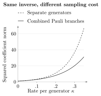
For equal $X,Y,Z$ generator rates, combining identical Pauli corrections reduces the squared coefficient norm from $e^{12\kappa}$ to $[(3e^{4\kappa}-1)/2]^2$. The physical noise and target are unchanged. These are bounded-outcome sampling scales; they omit characterization and execution costs.

Imperfect models leave bias

For an approximate circuit decomposition, write

$\mathcal C=\sum_aq_a\widetilde{\mathcal C}_a+\Delta.$

For normalized input and bounded $O$, the remaining expectation error obeys

$$\begin{aligned} |\operatorname{Tr}[O\Delta(\rho)]| &\leq\lVert O\rVert_\infty\lVert\Delta(\rho)\rVert_1\\ &\leq\lVert O\rVert_\infty\lVert\Delta\rVert_\diamond. \end{aligned}$$

Here the diamond norm has no factor of one half. A discrepancy measured on a few states and observables is not automatically a uniform norm bound.

If the true bit-flip probability is $.1$ but the fitted value is $.08$, the noisy mean $.48$ is corrected to $.48/.84=4/7$. The residual bias is $-1/35\simeq-.02857$. More science shots do not remove it.

Finite calibration also produces uncertainty. Hold the true physical distribution fixed while varying the estimated rate: the mean correction $m_{\rm obs}/(1-2\widehat p)$ has derivative $2m_{\rm obs}/(1-2\widehat p)^2$. At the true parameters in the example this is $1.5$. Independent binomial calibration with $M$ shots has variance $.09/M$, giving leading calibration contribution $.2025/M$ to the corrected mean’s variance. A common calibration creates covariance between separately estimated observables. The exact law of total variance separates conditional science variance from variance of the calibration-dependent conditional mean; the derivative formula is only a local approximation.

Test the complete sampled procedure on representative known-answer circuits and observables distinct from those used to tune it. Include phase-sensitive tests when coherent errors may matter. Preparation, readout, leakage and the inserted corrections must be modeled consistently; measurement-error mitigation treats terminal detector response separately.

If a variant succeeds with probability $a_j$, retaining only successful runs changes its frequency from $\pi_j$ to $\pi_ja_j/\sum_k\pi_ka_k$. The old signed weights no longer prove unbiasedness. Physical survival, numerical rejection and job failures need different models; none can silently disappear from normalization or cost. Likewise, symmetry conditioning introduces a ratio of signed sums, rather than an ordinary positive accepted fraction.

Exercises

1. Invert a mostly reversed bit-flip channel

Find the inverse coefficients, norm and sampling signs at $p=.8$. Compare with $p=1/2$ and $p=1$.

Solution

The coefficients are $(-1/3,4/3)$, with norm $5/3$, sampling probabilities $(.2,.8)$ and signs $(-,+)$. At $1/2$ the $Y,Z$ directions are erased. At one, the sole correction is $X$ with norm one. A high flip probability is not itself an information-loss criterion when the flip is predictable.

2. Derive an importance-sampling estimator

For any $\pi_a>0$ on the nonzero coefficients, prove unbiasedness of $X=q_a o/\pi_a$ and minimize its second moment over $\pi$.

Solution

Summing over the sampled label gives $\mathbb EX=\sum_aq_a\mu_a$. The second moment is $\sum_a q_a^2m_{2,a}/\pi_a$, where $m_{2,a}=\mathbb E[o^2|a]$. Cauchy–Schwarz gives minimum $(\sum_a|q_a|\sqrt{m_{2,a}})^2$, attained at $\pi_a\propto|q_a|\sqrt{m_{2,a}}$. Terms with zero second moment contribute nothing and can be omitted for that observable.

3. Move a correction through Hadamard

For the example in the text, explain why an $X$-noise inverse moved before Hadamard without modification fails. Which noise axis should the moved inverse use?

Solution

An $X$ inverse leaves $|+\rangle$ unchanged, so later $X$ noise still gives $.8$. Since $HXH=Z$, the correction moved through Hadamard must be the corresponding $Z$ inverse. Then $\mathcal N_X\mathcal H\mathcal N_Z^{-1}=\mathcal H$ in the exact model. Its physical implementation must still realize the assumed map.

4. Compose three sampling norms

For independent local bit-flip decompositions with $p=(.02,.05,.08)$, compute $\Gamma$ and a conservative shot count for standard error at most $.02$ with unit-bounded outcomes.

Solution

The norms are $25/24$, $10/9$ and $25/21$. Hence $\Gamma=3125/2268$ and $\Gamma^2=9765625/5143824\simeq1.89851$. The variance bound requires $N\geq\lceil\Gamma^2/.02^2\rceil=4747$. This bounds standard deviation, not a specified confidence level or systematic bias.

5. Compare bias with sampling uncertainty

At true $p=.1$, fitted $p=.08$ and ideal mean $.6$, calculate the residual bias. At the true fitted rate, compare leading calibration variance for $M=1000$ with science variance for $N=10000$.

Solution

The wrong-rate mean is $4/7$, with bias $-1/35$. For correctly centered calibration the leading variance is $.2025/1000=.0002025$, exceeding the exact-model science contribution $1.2025/10000=.00012025$. A narrow conditional science interval can therefore omit a larger uncertainty source, as well as any model bias.

6. Combine the three Pauli-generator inverses

Derive the combined coefficients in the figure and show that their norm is no greater than the factorized norm.

Solution

The inverse transfer eigenvalues are $(1,t,t,t)$ with $t=e^{4\kappa}$. Their Pauli transform gives $q_I=(1+3t)/4$ and the three remaining coefficients $(1-t)/4$. Let $x=e^{2\kappa}\geq1$. The norm difference is

$x^3-\frac{3x^2-1}{2}=\frac{(x-1)^2(2x+1)}2\geq0.$

Combining branches cancels some signed coefficients before sampling; it does not change the represented channel.

7. Detect a missing nonunital direction

Amplitude damping has affine Bloch action $r\mapsto Dr+t$ with $t\ne0$ and invertible $D$. Can its full inverse be a normalized real linear combination of Pauli conjugations?

Solution

The inverse maps $r$ to $D^{-1}r-D^{-1}t$, so it has a nonzero translation. Every Pauli conjugation is unital, and any trace-preserving real combination has coefficients summing to one and remains unital. It cannot reproduce that translation. Channel invertibility alone therefore does not supply a feasible Pauli-only inverse decomposition.

8. Check survival-dependent sampling

Two branches are requested with probabilities $(.9,.1)$ and succeed with probabilities $(1,.5)$. What law do retained labels follow, and why can the original PEC weights fail?

Solution

Overall success is $.95$ and the retained law is $(18/19,1/19)$, not $(.9,.1)$. In general the weighted branch means are therefore combined with different coefficients. Correcting label frequencies alone would still require success to leave the relevant within-branch outcome distribution unchanged; state-dependent physical loss needs its full conditional model.

References

• Z. Cai, R. Babbush, S. C. Benjamin, S. Endo, W. J. Huggins, Y. Li, J. R. McClean, and T. E. O’Brien, “Quantum Error Mitigation,” Reviews of Modern Physics 95, 045005 (2023), doi:10.1103/RevModPhys.95.045005 — broader context and experimental limitations.
• S. Endo, S. C. Benjamin, and Y. Li, “Practical Quantum Error Mitigation for Near-Future Applications,” Physical Review X 8, 031027 (2018), doi:10.1103/PhysRevX.8.031027.
• C. Piveteau, D. Sutter, and S. Woerner, “Quasiprobability Decompositions with Reduced Sampling Overhead,” npj Quantum Information 8, 12 (2022), doi:10.1038/s41534-022-00517-3.
• K. Temme, S. Bravyi, and J. M. Gambetta, “Error Mitigation for Short-Depth Quantum Circuits,” Physical Review Letters 119, 180509 (2017), doi:10.1103/PhysRevLett.119.180509.
• E. van den Berg, Z. K. Minev, A. Kandala, and K. Temme, “Probabilistic Error Cancellation with Sparse Pauli–Lindblad Models on Noisy Quantum Processors,” Nature Physics 19, 1116–1121 (2023), doi:10.1038/s41567-023-02042-2.