Leakage and Crosstalk

Leakage moves amplitude outside the states used for a computational encoding. Crosstalk makes operations on different hardware regions fail to behave independently. They can interact: a leaked level may persist and change a neighbor’s phase. Modeling either effect requires retaining the physical degrees of freedom that influence the next operation, rather than replacing every error by a trace-preserving qubit map.

Helpful background. Direct sums versus tensor products distinguishes alternative sectors of one system from simultaneous subsystems. Quantum channels and instruments provide the linear maps and outcome probabilities used below.

Computational sectors and retained states

Choose a projector $P$ onto the computational states and put $Q=I-P$. Then

$$\begin{gathered} \mathcal H=\mathcal H_C\oplus\mathcal H_L,\\ d_C=\operatorname{Tr}P,\quad d_L=\operatorname{Tr}Q. \end{gathered}$$

The two sectors are alternatives within one system. A third circuit level may be leakage for a qubit encoding and an intended state for a qutrit encoding. The direct sum permits coherence between sectors; it is not a superselection rule. Also distinguish physical carrier leakage from leaving a many-qubit error-correcting code space: a correctable Pauli fault can leave that code space while every carrier remains in its intended two levels. Leakage-tolerant fault correction must account for the larger physical space (Aliferis and Terhal, 2007).

Let $\mathcal E$ be CPTP on the full physical space. For a normalized input supported in $P$, the computational-survival operation is

$$\begin{aligned} \mathcal C(\rho)&=P\mathcal E(\rho)P,\\ a(\rho)&=\operatorname{Tr}\mathcal C(\rho),\\ p_L(\rho)&=1-a(\rho)=\operatorname{Tr}[Q\mathcal E(\rho)]. \end{aligned}$$

$\mathcal C$ is completely positive and trace nonincreasing. If survival is physically selected and $a>0$, its conditional state is $\mathcal C(\rho)/a(\rho)$. This normalization is generally nonlinear. For $K=\operatorname{diag}(1,1/\sqrt2)$, the retained operation $K\rho K^\dagger$ takes $I/2$ to a branch with trace $3/4$ and conditional state $\operatorname{diag}(2/3,1/3)$. In contrast, equally mixing the separately normalized basis-state outputs gives $I/2$. Keep the branch probability when combining runs or further operations.

Selecting survival is also different from forgetting a flag. Summing all outcome branches is trace preserving; retaining only the successful branch may lose trace. A flag alone does not make a process a standard erasure channel: loss can depend on the input, and surviving amplitudes can be filtered.

Average, state-dependent and worst-case leakage

For nonzero sector dimensions, Wood and Gambetta (2018) define average leakage and seepage by maximally mixed sector inputs:

$$\begin{aligned} L_1&=\operatorname{Tr}[Q\mathcal E(P/d_C)],\\ L_2&=\operatorname{Tr}[P\mathcal E(Q/d_L)]. \end{aligned}$$

Seepage means return from $Q$ to $P$, not recovery of the original logical state. With Kraus operators $K_\alpha$,

$$\begin{aligned} L_1&=d_C^{-1}\sum_\alpha\|QK_\alpha P\|_F^2,\\ L_2&=d_L^{-1}\sum_\alpha\|PK_\alpha Q\|_F^2. \end{aligned}$$

The maximum escape probability over computational inputs is instead

$L_{\max}=\lambda_{\max}[P\mathcal E^\dagger(Q)P].$

This follows because $p_L(\rho)$ is the expectation of that positive effect. For a full-space unitary, $L_{\max}=\|QUP\|_{\mathrm{op}}^2$. Average and worst-case values need not agree.

Unital channels satisfy $d_CL_1=d_LL_2$, but unitality is sufficient, not necessary. For every trace-preserving map,

$d_CL_1-d_LL_2=\operatorname{Tr}[Q\mathcal E(I)]-d_L.$

Thus balance only constrains one sector trace of $\mathcal E(I)$. It does not establish $\mathcal E(I)=I$. Reset and thermalization generally violate balance, but some nonunital maps satisfy it for a particular sector split; exercise2 gives a counterexample.

Coherent escape, return and measurement

Use basis $(|0\rangle,|1\rangle,|\ell\rangle)$ with the first two states computational, and the real rotation

$$U_\theta=\begin{pmatrix} 1&0&0\\0&\cos\theta&-\sin\theta\\0&\sin\theta&\cos\theta \end{pmatrix}.$$

Only $|1\rangle$ couples to the leakage level. Consequently

$$\begin{aligned} p_L(|0\rangle)&=0,\qquad p_L(|1\rangle)=\sin^2\theta,\\ L_1&=\tfrac12\sin^2\theta,\\ L_2&=L_{\max}=\sin^2\theta. \end{aligned}$$

At $\theta=0.2$, state leakage from $|1\rangle$ is approximately $0.039470$, while the computational average is $0.019735$. Neither is “the leakage probability” independently of the input.

Define sector dephasing by $\Delta(\rho)=P\rho P+Q\rho Q$. A useful coherence measure, with no factor of $1/2$, is

$$\begin{aligned} C_L(\rho)&=\|\rho-\Delta(\rho)\|_1,\\ 0\leq C_L(\rho)&\leq2\sqrt{p_Cp_L}\leq1. \end{aligned}$$

For $U_\theta|1\rangle$ it is $|\sin2\theta|$, approximately $0.389418$ at the chosen angle. It measures coherence, not escape probability.

Two same-sign pulses produce leakage $\sin^2(2\theta)$. An exact inverse pulse instead returns the original state with zero leakage. Now measure the sector after the first pulse, discard the result, and apply the inverse. The intermediate dephasing removes the interference needed for perfect return, leaving

$p_L=2\sin^2\theta\cos^2\theta.$

At $\theta=0.2$, these three outcomes are respectively $0.151647$, $0$ and $0.075823$.

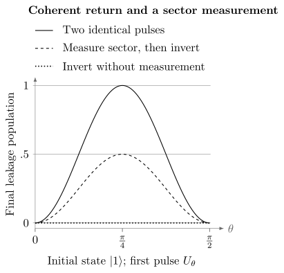
Start in $|1\rangle$ and apply $U_\theta$. A second identical pulse gives $\sin^2(2\theta)$ (solid). An inverse pulse gives zero (dotted), but an intervening unread projective sector measurement raises that result to $\tfrac12\sin^2(2\theta)$ (dashed). The flag changes the experiment even when its classical result is discarded.

Zero final leakage also need not mean a correct logical operation. Let $S$ swap $|1\rangle$ and $|\ell\rangle$, fixing $|0\rangle$, and let $V_\varphi=P+e^{i\varphi}Q$. Then $SV_\varphi S$ returns every computational input but acts there as $\operatorname{diag}(1,e^{i\varphi})$. On $|+\rangle$, final $(X,Y)$ expectations are $(\cos\varphi,\sin\varphi)$. A final population check misses this phase. A sector measurement during the excursion also destroys the superposition’s cross-sector coherence.

What a leakage detector specifies

An ideal projective sector detector after $\mathcal E$ has operations

$$\begin{aligned} \mathcal I_C(\rho)&=P\mathcal E(\rho)P,\\ \mathcal I_L(\rho)&=Q\mathcal E(\rho)Q. \end{aligned}$$

Forgetting its result gives $\Delta\circ\mathcal E$, which need not equal the unmeasured process. An imperfect detector is often modeled as classical mislabeling of this sector outcome. With sector-independent false-positive and false-negative probabilities $f_p,f_n$,

$$\begin{aligned} p_{\mathrm{flag}}&=f_p+(1-f_n-f_p)p_L,\\ p_L&=\frac{p_{\mathrm{flag}}-f_p}{1-f_n-f_p}. \end{aligned}$$

This response formula assumes effect $F_{\mathrm{flag}}=f_pP+(1-f_n)Q$. Calibration on two sector averages does not establish that form for every coherent input or every state inside a multidimensional sector. At $f_p+f_n=1$ the detector carries no sector information; a small denominator amplifies statistical and calibration error.

Even a known effect fixes only outcome probabilities, not the postmeasurement state. Different instruments with that effect can produce different later leakage and return. To predict a detector followed by further gates, characterize or model its backaction as well as its classification errors (Varbanov et al., 2020).

When populations alone are enough

A full map closes exactly on the two sector populations for every input if and only if

$\mathcal E^\dagger(Q)=L_1P+(1-L_2)Q.$

Taking expectations yields

$p_{L,m+1}=L_1+(1-L_1-L_2)p_{L,m}.$

The condition excludes both state dependence within a sector and coherence feeding into the next population. The coherent rotation above does not satisfy it: $|0\rangle$ and $|1\rangle$ have different escape probabilities. Randomization can justify an averaged population model, but that is a statement about the specified ensemble.

For constant rates with $L_1+L_2>0$, put $q=1-L_1-L_2$ and $p_L^*=L_1/(L_1+L_2)$. Then

$p_{L,m}=p_L^*+q^m[p_{L,0}-p_L^*].$

This is a limit from every initial population only when $|q|<1$. Negative $q$ permits alternating convergence, and $L_1=L_2=1$ gives a period-two swap. Both rates zero leave every population stationary. See common noise models for the derivation.

For $L_1=0.02$, $L_2=0.18$, initially $p_L=0$, the exact solution is $p_L(m)=0.1(1-0.8^m)$. With $f_p=0.01$, $f_n=0.05$, the predictions are:

Cycle	Leakage population	Flag probability
$0$	$0$	$0.010000$
$1$	$0.020000$	$0.028800$
$2$	$0.036000$	$0.043840$
$5$	$0.067232$	$0.073198$
$10$	$0.089263$	$0.093907$

Values are rounded to six decimals. A possible full qutrit realization is

$$\begin{aligned} K_0&=\sqrt{0.98}P+\sqrt{0.82}Q,\\ K_1&=\sqrt{0.02}|\ell\rangle\langle0|,\\ K_2&=\sqrt{0.02}|\ell\rangle\langle1|,\\ K_3&=\sqrt{0.09}|0\rangle\langle\ell|,\\ K_4&=\sqrt{0.09}|1\rangle\langle\ell|. \end{aligned}$$

It is trace preserving, has the stated closed populations, and is nonunital. Other realizations can have identical population dynamics but different retained coherence. In hardware, leaked-level persistence can also mediate later correlated errors, as demonstrated in a superconducting correction experiment by McEwen et al. (2021). A single fitted leakage number cannot describe that entire process.

Crosstalk across simultaneously present regions

Distinct regions use tensor factors, for example

$\mathcal H_{AB}=(\mathcal H_{C,A}\oplus\mathcal H_{L,A})\otimes\mathcal H_B.$

During a layer with no intended interaction, a strict independent model has

$\mathcal E_{s_A,s_B}=\mathcal E_{A,s_A}\otimes\mathcal E_{B,s_B}.$

Each local channel depends only on its own instruction. A joint nonproduct channel violates locality; changing a remote instruction can also reveal context dependence. These are operational notions of crosstalk (Sarovar et al., 2020). An intended entangling gate is outside this independent-layer model. If shared noise is explicitly allowed, one is testing a broader model and should not identify it with the strict product assumption.

With independently prepared inputs and trusted local readout, the product model implies

$p(a,b\mid s_A,s_B)=p_A(a\mid s_A)p_B(b\mid s_B).$

Correlated preparation, correlated readout or drift can also violate this observed relation, so a probability correlation alone does not identify a dynamical mechanism. Interleave settings in time and compare the same local instruction with the remote region idle, driven, measured and reset (Rudinger et al., 2019). Device characterization discusses calibration and uncertainty; error-aware compilation discusses scheduling responses.

For fixed product spectator input $\sigma_B$, the target’s reduced map is

$$\mathcal E_{A\mid s_B,\sigma_B}(\rho_A) =\operatorname{Tr}_B\mathcal E_{s_A,s_B}(\rho_A\otimes\sigma_B).$$

It is CPTP. Initial target–spectator correlations, or a spectator retaining information from earlier gates, can prevent reuse of one such state-independent map. Compare observable probabilities or consistently reconstructed models, rather than interpreting a gauge-dependent tomography coefficient as a uniquely measured coupling.

Two different ZZ mechanisms

A residual interaction

$U_{ZZ}(\phi)=e^{-i\phi Z_AZ_B/2}$

rotates A by $+\phi$ or $-\phi$ when B is a $Z$ eigenstate. Equal averaging over those spectator states gives one-step coherence $\cos\phi$. Persistence changes repetition:

Spectator preparation	Target coherence after $m$ intervals
One random sign retained throughout	$\cos(m\phi)$
Independent equal re-preparation each time	$(\cos\phi)^m$
Fixed known eigenvalue $b=\pm1$	$e^{-ibm\phi}$

At $\phi=0.12$, $m=8$, the first two real coherences are approximately $0.573520$ and $0.943896$. They share the same one-step map. Replacing a persistent spectator by independent Pauli draws would miss this difference.

A distinct example is the stochastic joint channel

$\Phi_p(\rho)=(1-p)\rho+pZ_AZ_B\rho Z_AZ_B.$

On $|++\rangle$,

$$\begin{aligned} \langle X_A\rangle&=\langle X_B\rangle=1-2p,\\ \langle X_AX_B\rangle&=1. \end{aligned}$$

At $p=0.1$, the connected expectation is $1-0.8^2=0.36$. Under trusted product preparation/readout, this rejects the product channel. Yet A’s marginal channel is $(1-p)\rho_A+pZ_A\rho_AZ_A$, independent of B’s input. Thus the absence of remote signaling or a changed local marginal does not establish a product channel. This fixed correlated channel needs no varied context to fail locality.

Exercises

1. Complete a survival filter

Embed $K=\operatorname{diag}(1,1/\sqrt2)$ into a trace-preserving qutrit channel and compare normalization before and after mixing the two basis preparations.

Solution

Take $\widetilde K=\operatorname{diag}(1,1/\sqrt2,1)$ and $K_f=|\ell\rangle\langle1|/\sqrt2$. Their effects sum to $I_3$. For a computational input the survival probability is $\rho_{00}+\rho_{11}/2$.

For $I/2$, survival has probability $3/4$ and conditional state $\operatorname{diag}(2/3,1/3)$. Each basis input separately survives as itself, so their equally weighted conditional mixture is $I/2$. The trace distance between these matrices is $1/6$. Actual accepted samples have weights proportional to their survival probabilities, not equal weights.

2. Test the balance condition

Derive the general flux identity and show that it does not imply unitality. Use a qutrit reset to $|v\rangle=\sqrt{2/3}|0\rangle+\sqrt{1/3}|\ell\rangle$.

Solution

Since $\operatorname{Tr}\mathcal E(Q)=d_L$,

$$\begin{aligned} d_CL_1-d_LL_2 &=\operatorname{Tr}[Q\mathcal E(P)]-\operatorname{Tr}[P\mathcal E(Q)]\\ &=\operatorname{Tr}[Q\mathcal E(I)]-d_L. \end{aligned}$$

For the reset channel, $\mathcal E(I_3)=3|v\rangle\langle v|\ne I_3$, but its leakage-sector trace is one. Directly $L_1=1/3$, $L_2=2/3$, and $d_C=2,d_L=1$ give $d_CL_1=d_LL_2=2/3$. Sector balance holds without unitality.

3. Derive average and worst-case leakage

For $U_\theta$, find the leakage effect on the computational sector and derive $L_1,L_2,L_{\max}$. Compare with the input $|+\rangle$.

Solution

$PU_\theta^\dagger QU_\theta P=\sin^2\theta|1\rangle\langle1|$. Its average on $P/2$ is $\sin^2\theta/2$ and its largest eigenvalue is $\sin^2\theta$. Starting in $|\ell\rangle$ returns with probability $\sin^2\theta$, so $L_2$ equals the latter. The plus input has population $1/2$ in the coupled direction and therefore leakage $\sin^2\theta/2$, but its surviving state is coherently filtered rather than unchanged.

4. Compare reversal and a measured excursion

Starting from $|1\rangle$, compare $U_\theta^\dagger U_\theta$ with $U_\theta$, an unread sector measurement, and then $U_\theta^\dagger$. Separately explain how $SV_\varphi S$ can have zero final leakage but a logical error.

Solution

The first sequence is identity. The measured intermediate state is $\cos^2\theta|1\rangle\langle1|+\sin^2\theta|\ell\rangle\langle\ell|$. After the inverse pulse both branches contribute $\sin^2\theta\cos^2\theta$ to leakage, giving $\tfrac12\sin^2(2\theta)$.

The swap–phase–swap path instead produces $\operatorname{diag}(1,e^{i\varphi})$ within the code. Final population is fully restored, but a plus input has equatorial phase $\varphi$. Measuring the sector during that excursion dephases the plus superposition; on the basis input $|1\rangle$ alone that measurement is deterministic and does not cause such dephasing.

5. Predict and invert a flag rate

For the tabulated population model, compute cycle-five leakage and the imperfect flag probability. Explain why the classical flag formula does not determine later quantum states.

Solution

$p_L(5)=0.1(1-0.8^5)=0.067232$. The flag rate is $0.01+0.94p_L=0.07319808$, so $(p_{\mathrm{flag}}-0.01)/0.94$ recovers the leakage. An effect determines these probabilities, but an instrument also determines the state update. A detector can, for example, apply an additional unitary after each outcome without changing either effect, yet change later interference.

6. Derive persistent-spectator coherence

Derive the three coherence factors in the ZZ table. How can a reset comparison distinguish them?

Solution

For spectator eigenvalue $b$, one interval multiplies target coherence by $e^{-ib\phi}$. Retaining the same random sign for all intervals gives $\tfrac12(e^{-im\phi}+e^{im\phi})=\cos(m\phi)$. Independent equal redraws average each factor separately, giving $(\cos\phi)^m$. A known fixed sign gives $e^{-ibm\phi}$ with no attenuation.

Interleave no-reset, random-repreparation and known-state-reset experiments and measure both quadratures versus depth. Reset errors and drift must be included in the comparison; the three ideal laws are predictions of the stated spectator model, not universal reset behavior.

7. Distinguish joint noise from its marginals

Compare $\Phi_p$ with independent local phase flips having the same marginal probability $p$. On $|++\rangle$, compute both joint $XX$ expectations and explain the role of preparation/readout assumptions.

Solution

Each channel gives local $X$ expectations $1-2p$. The joint channel applies either $II$ or $ZZ$, both of which preserve $XX$, so its joint expectation is one. Independent flips give $(1-2p)^2$. At $p=0.1$ the difference is $0.36$.

This distinguishes the channels with trusted product input and local readout. An initially correlated state or correlated readout can mimic the same statistical signature, so the comparison alone does not identify a residual Hamiltonian or other microscopic cause.

References

• P. Aliferis and B. M. Terhal, “Fault-tolerant quantum computation for local leakage faults,” Quantum Information and Computation 7, 139–156 (2007), doi:10.26421/QIC7.1-2-9.
• M. McEwen, D. Kafri, Z. Chen, et al., “Removing leakage-induced correlated errors in superconducting quantum error correction,” Nature Communications 12, 1761 (2021), doi:10.1038/s41467-021-21982-y.
• K. Rudinger, T. Proctor, D. Langharst, M. Sarovar, K. Young, and R. Blume-Kohout, “Probing context-dependent errors in quantum processors,” Physical Review X 9, 021045 (2019), doi:10.1103/PhysRevX.9.021045.
• M. Sarovar, T. Proctor, K. Rudinger, K. Young, E. Nielsen, and R. Blume-Kohout, “Detecting crosstalk errors in quantum information processors,” Quantum 4, 321 (2020), doi:10.22331/q-2020-09-11-321.
• B. M. Varbanov, F. Battistel, B. M. Tarasinski, V. P. Ostroukh, T. E. O’Brien, L. DiCarlo, and B. M. Terhal, “Leakage detection for a transmon-based surface code,” npj Quantum Information 6, 102 (2020), doi:10.1038/s41534-020-00330-w.
• C. J. Wood and J. M. Gambetta, “Quantification and characterization of leakage errors,” Physical Review A 97, 032306 (2018), doi:10.1103/PhysRevA.97.032306.