Dynamical Decoupling in Quantum Circuits

Dynamical decoupling (DD) uses control pulses to reduce unwanted evolution while a qubit stores or processes information. It is particularly useful when noise changes slowly enough for the control to reverse its accumulated effect. Real pulses also introduce errors, so the best sequence is the one that preserves the desired quantum operation under the available timing, calibration and noise conditions.

This page applies DD to idle intervals and computation: how to preserve the intended operation, fit pulses into a schedule and compare the resulting performance. The general dynamical-decoupling lesson develops the sequence and filter theory. DD changes the physical channel before measurement; it does not infer an ideal answer from noisy records or perform syndrome-based recovery.

Required background. Noise and mitigation distinguishes physical suppression from estimation. Dynamical decoupling introduces toggling frames and refocusing.

Helpful background. Pulse sequences describes sequence families; average Hamiltonian theory explains controlled evolution; variance and covariance supports the paired comparison below.

Preserve the intended operation

An idle means identity in a specified rotating or logical frame. Laboratory-frame precession may be intentional, and a virtual frame update changes the axes of later pulses. Always compare the entire controlled interval with its intended operation in the same frame.

Write an ideal rotation as $R_x(\theta)=e^{-i\theta X/2}$. If pulses $P_1,\ldots,P_N$ occur in chronological order, their product acts right-to-left. For a protected idle, the pulse-only requirement is

$P_N\cdots P_1=e^{i\phi}I.$

Four $X_\pi=-iX$ pulses give identity; two give $-I$. One uncompensated $X_\pi$ pulse does not preserve an arbitrary input, even when it refocuses dephasing. An echo experiment can account for that known rotation in its readout or frame convention. The phase above is harmless only if it is global over the entire relevant space; different phases on leakage states or coherently controlled branches can matter.

The pulse product alone does not test evolution between or during pulses. For a gate, the complete product must implement the target gate, rather than merely end with an identity pulse cycle. A simple warning is a desired static $Z$ rotation: the same balanced echo that removes a nuisance $Z$ detuning also removes that rotation. Preserving useful dynamics while canceling errors requires appropriately designed control, not arbitrary insertion of an idle sequence.

The group-averaging formulation of Viola, Knill and Lloyd (1999) explains how control can suppress selected interaction terms. Higher-order effects and finite pulses require additional analysis; there is no universal sequence that cancels arbitrary noise without changing the task.

Turn pulse times into a physical schedule

A pulse with center $t_j$ and duration $\tau_j$ occupies $[t_j-\tau_j/2,t_j+\tau_j/2]$. Check those edges against neighboring operations, waveform tails, minimum free gaps and shared drive or coupler resources. A center inside an idle is insufficient if part of its pulse lies outside.

For a concrete example, take a $1200\,\mathrm{ns}$ idle, four requested centers $(150,450,750,1050)\,\mathrm{ns}$, a nearest $8\,\mathrm{ns}$ timing grid and $40\,\mathrm{ns}$ pulses:

Pulse	Realized center (ns)	Occupied interval (ns)
1	152	132–172
2	448	428–468
3	752	732–772
4	1048	1028–1068

The free gaps are $(132,256,264,256,132)\,\mathrm{ns}$. They satisfy a $100\,\mathrm{ns}$ boundary guard and $250\,\mathrm{ns}$ minimum internal gap. The pulse duty fraction is $160/1200\simeq13.3\%$. These geometric checks say that the schedule fits; they do not establish noise suppression.

In an instantaneous-pulse approximation, $y(t)=(-1)^{n(t)}$ changes sign at each pulse center. For static detuning $\xi_0$, the remaining phase is $\xi_0Y(0)$, where $Y(0)=\int_0^T y(t)\,dt$. The requested times give zero, but the rounded schedule gives

$$\begin{aligned} Y(0)&=152-296+304-296+152\\ &=16\,\mathrm{ns}. \end{aligned}$$

Thus its normalized static residual is about $1.33\%$. The timing grid has changed the cancellation even though the ideal pulse product and spacing tests still pass. Use the emitted times, including any inserted frame updates, when predicting behavior. Pulse-level control explains the schedule representation.

During a finite pulse, $U_c^\dagger(t)ZU_c(t)$ generally rotates continuously and has several Pauli components. Replacing it by $y(t)Z$ throughout the pulse is not exact. Integrate the control Hamiltonian, or state and justify a strong-control or negligible-pulse-duration approximation. Leakage and spectator disturbance need a larger model than this two-level one.

Check which noise the schedule suppresses

For $H_{\rm noise}(t)=\xi(t)Z/2$ in units with $\hbar=1$, a zero-mean stationary classical Gaussian fluctuation gives coherence $C=e^{-\chi}$ under ideal sign modulation. Fix the spectral convention by

$$\begin{aligned} \langle\xi(t)\xi(0)\rangle &=\int_{-\infty}^{\infty}\frac{d\omega}{2\pi} S_{\xi\xi}(\omega)e^{-i\omega t},\\ Y(\omega,T)&=\int_0^T y(t)e^{i\omega t}\,dt,\\ \chi&=\frac12\int_{-\infty}^{\infty}\frac{d\omega}{2\pi} S_{\xi\xi}(\omega)|Y(\omega,T)|^2. \end{aligned}$$

Here $\xi$ has units $\mathrm{s}^{-1}$, $Y$ has units $\mathrm{s}$, and $S_{\xi\xi}$ has units $\mathrm{s}^{-1}$, making $\chi$ dimensionless. The factor $1/2$ comes from the Gaussian characteristic function. Non-Gaussian noise generally needs more than its two-point spectrum. Cywiński et al. (2008) study both Gaussian descriptions and strongly coupled fluctuators.

A low-frequency zero suppresses only the spectral contributions it actually overlaps. Moving weight away from low frequencies can move it toward another noise band. A high-order zero of a filter is also distinct from cancellation order in a Magnus expansion; Paz-Silva and Viola (2014) develop this distinction. Neither theoretical order alone ranks experimental performance.

White dephasing and relaxation

If $\langle\xi(t)\xi(t')\rangle=2\gamma\delta(t-t')$, then

$\chi=\gamma\int_0^T y(t)^2dt=\gamma T.$

Ideal sign reversals cannot reduce this white-noise exposure. Equivalently, changing $Z$ to $-Z$ leaves the Markovian dissipator unchanged. This statement assumes ideal instantaneous modulation and that same noise model; it does not cover every possible driven open system.

Unitary pulses also cannot reverse an unknown amplitude-damping jump. They may change the coupling or effective relaxation in a structured environment, but that needs an explicit physical model. To illustrate a remaining relaxation cost, suppose a phenomenological channel has transverse contraction $\sqrt\eta C$ and longitudinal contraction $\eta=e^{-T/T_1}$. Its average input-state fidelity is

$F_{\rm avg}=\frac{3+\eta+2\sqrt\eta C}{6}.$

At $T=20\,\mu\mathrm{s}$ and $T_1=60\,\mu\mathrm{s}$, changing $C$ from $e^{-20/12}$ to $e^{-20/45}$ raises this fidelity from $.673$ to $.800$. Even $C=1$ gives only $.902$. This comparison assumes unchanged amplitude damping; it is not the channel automatically generated by applying $X$ pulses during relaxation. Such pulses can rotate damping into excitation in the toggling frame.

Include coherent pulse errors

More pulses can improve environmental refocusing while worsening control error. Consider four instantaneous pulses, no environmental evolution, perfect axes and the same angle error $\epsilon$ on every pulse. Four $x$ pulses implement a residual rotation by $4\epsilon$ after removing their ideal identity. Their average infidelity is

$r_{XXXX}=\frac{1-\cos(4\epsilon)}3.$

For chronological axes $x,y,x,y$, the product is

$$\begin{aligned} \theta&=\pi+\epsilon,\\ U_{XYXY}&=[R_y(\theta)R_x(\theta)]^2. \end{aligned}$$

It is $-I$ at $\epsilon=0$. Let $q=\sin(\epsilon/2)$. Direct multiplication gives

$r_{XYXY}=\frac83q^4(1-q^4).$

The leading errors are $8\epsilon^2/3$ and $\epsilon^4/6$, respectively. At $\epsilon=.1$ radians they are about $.0263$ and $1.66\times10^{-5}$. Both sequences have four pulses, but their coherent errors combine differently.

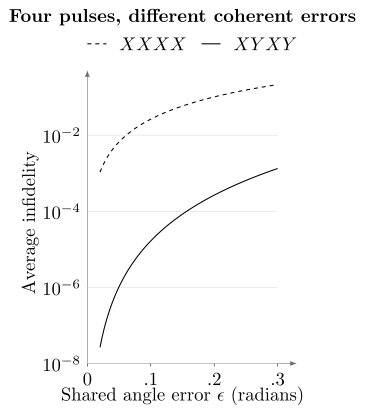
Exact two-level pulse products in the stated angle-error model. Alternating axes cancels the leading coherent error; the vertical axis is logarithmic. Environmental noise, detuning errors and finite pulse widths are absent, so the plot does not establish a universal sequence ranking.

A state aligned with the residual rotation axis can look perfectly preserved while other states fail. This is why a single favorable survival probability does not establish arbitrary-state protection. Souza, Álvarez and Suter (2011) and Wang et al. (2012) analyze pulse-error robustness in more realistic settings. Ezzell et al. (2023) also show why pulse spacing and device context matter in experimental comparisons.

Compare performance at equal resources

Measure the quantity the application needs: coherence of a particular state, average or worst-state memory fidelity, or an algorithmic observable. A longer fitted $T_2$ is useful but does not establish all of these. Include leakage, loss and spectator effects; conditioning on surviving computational states can hide increased failure.

Interleave baseline and DD measurements in matched time blocks to reduce drift confounding. Select the sequence on separate data, then evaluate the chosen sequence on fresh states or circuits. With matched quality scores $b_i,d_i$, calculate differences $\delta_i=d_i-b_i$ and use their sample variance:

$$\begin{aligned} \overline\delta&=\frac1m\sum_i\delta_i,\\ \operatorname{SE}(\overline\delta)&=\frac{s_\delta}{\sqrt m}. \end{aligned}$$

For baseline scores $(.78,.80,.76,.81,.77,.79)$ and DD scores $(.88,.87,.83,.89,.80,.86)$, the mean gain is $.070$ and its paired standard error is $.00931$. Treating the records as independent gives $.0158$. A Student-$t$ interval is approximately $[.0461,.0939]$ if the six block differences are independent and approximately normally distributed. Pairing does not justify that distributional assumption or remove correlations between blocks.

Count calibration and tuning runs as well as final shots. If pulses lengthen the circuit, either compare with an equal-duration baseline or include the extra time in the resource comparison. Added drive power, occupied hardware and recalibration can outweigh a small gain. Keeping the original idle can be the better choice.

Combining DD with extrapolation or probabilistic cancellation changes the noise those estimators encounter. Check the actual combined circuits: scaling durations can change DD timing, and a cancellation model for an unprotected gate need not apply after protection. A readout response need only be recalibrated if it changes or its transfer is uncertain; physical suppression does not automatically alter every downstream detector parameter.

Exercises

1. Track the ideal net action

Compute the products of two and four ideal $X_\pi$ pulses and of chronological $X_\pi,Y_\pi,X_\pi,Y_\pi$. Why is a single echo pulse insufficient for an arbitrary-state identity?

Solution

The first two products are $-I$ and $I$. The alternating product is $YXYX=-I$, including the four factors of $-i$. Each is identity up to a global phase. A single pulse is $-iX$, which swaps $|0\rangle$ and $|1\rangle$; its known action must be compensated or incorporated in the intended final frame or measurement.

2. Reconstruct the rounded schedule

Find the free gaps, duty fraction and static moment from the timing table. Does symmetric placement around the midpoint force zero static moment?

Solution

Subtract successive pulse edges and the window boundaries to get $(132,256,264,256,132)\,\mathrm{ns}$. Pulse occupancy is $4(40)=160\,\mathrm{ns}$, hence duty $2/15$. Instantaneous signed center intervals give $Y(0)=16\,\mathrm{ns}$. Reflection symmetry alone does not balance the total positive and negative durations for this even-pulse pattern.

3. Convert spectral units

A one-sided ordinary-frequency PSD obeys $\langle\xi^2\rangle=\int_0^\infty S_f^{(1)}(f)df$. Express the two-sided angular-frequency PSD used above.

Solution

For a real stationary process,

$S_{\xi\xi}(\omega)=\tfrac12S_f^{(1)}(|\omega|/(2\pi)).$

The half accounts for positive and negative frequencies. Since $d\omega/(2\pi)=df$, no extra $2\pi$ factor appears in this convention. A PSD integrated with $d\omega$ alone would have a different normalization.

4. Verify the coherent-error figure

Use $F_{\rm avg}(U,I)=(|\operatorname{Tr}U|^2+2)/6$ to derive both curves. Explain why multiplying individual pulse fidelities fails.

Solution

The same-axis product has trace $2\cos(2\epsilon)$, giving $r=(1-\cos4\epsilon)/3$. For the alternating product, let $c=\cos((\pi+\epsilon)/2)=-q$; its trace is $2(2c^4-1)$. Substitution gives $r=(8/3)q^4(1-q^4)$. Coherent rotations compose as amplitudes with signs and axes, not independent failure probabilities. For $N$ equal same-axis small errors, the leading infidelity is $N^2\epsilon^2/6$, rather than $N\epsilon^2/6$.

5. Distinguish dephasing suppression from relaxation

Derive the average fidelity of the phenomenological channel above. What prevents the value from reaching one when $C=1$?

Solution

For Bloch action $\boldsymbol r\mapsto A\boldsymbol r+\boldsymbol c$, average pure-input fidelity is $(3+\operatorname{Tr}A)/6$: spherical averaging gives $\langle r_ir_j\rangle=\delta_{ij}/3$ and $\langle\boldsymbol r\rangle=0$. Here $A$ has diagonal entries $(\sqrt\eta C,\sqrt\eta C,\eta)$. Even with $C=1$, $\eta<1$ contracts the Bloch sphere. Removing pure dephasing has not undone damping.

6. Check the paired uncertainty

Recompute the gain and standard error from the six pairs. What additional assumption enters the stated confidence interval?

Solution

The differences are $(.10,.07,.07,.08,.03,.07)$, with mean $.07$ and sample variance $.00052$. Thus the standard error is $\sqrt{.00052/6}=.00931$. Multiplying by $t_{.975,5}\simeq2.571$ gives half-width $.0239$. The exact Student-$t$ construction assumes independent normal differences; six pairs alone do not establish normality. Correlated blocks or same-data sequence selection require another analysis or new measurements.

References

• Ł. Cywiński, R. M. Lutchyn, C. P. Nave, and S. Das Sarma, “How to Enhance Dephasing Time in Superconducting Qubits,” Physical Review B 77, 174509 (2008), doi:10.1103/PhysRevB.77.174509.
• N. Ezzell, B. Pokharel, L. Tewala, G. Quiroz, and D. A. Lidar, “Dynamical Decoupling for Superconducting Qubits: A Performance Survey,” Physical Review Applied 20, 064027 (2023), doi:10.1103/PhysRevApplied.20.064027.
• G. A. Paz-Silva and L. Viola, “General Transfer-Function Approach to Noise Filtering in Open-Loop Quantum Control,” Physical Review Letters 113, 250501 (2014), doi:10.1103/PhysRevLett.113.250501.
• A. M. Souza, G. A. Álvarez, and D. Suter, “Robust Dynamical Decoupling for Quantum Computing and Quantum Memory,” Physical Review Letters 106, 240501 (2011), doi:10.1103/PhysRevLett.106.240501.
• L. Viola, E. Knill, and S. Lloyd, “Dynamical Decoupling of Open Quantum Systems,” Physical Review Letters 82, 2417–2421 (1999), doi:10.1103/PhysRevLett.82.2417.
• Z.-H. Wang, W. Zhang, A. M. Tyryshkin, S. A. Lyon, J. W. Ager, E. E. Haller, and V. V. Dobrovitski, “Effect of Pulse Error Accumulation on Dynamical Decoupling of the Electron Spins of Phosphorus Donors in Silicon,” Physical Review B 85, 085206 (2012), doi:10.1103/PhysRevB.85.085206.