Limits of Error Mitigation

Error mitigation can improve an expectation estimate while making its statistical uncertainty or calibration sensitivity much larger. Sometimes the available noisy data contain no information about the desired quantity at all. Understanding these limits helps distinguish a useful finite calculation from a promise of efficient recovery for arbitrary circuits.

The central questions are concrete: which ideal quantity is required, which noisy experiments are available, what error is acceptable, and how much total work can be spent? A lower bound answers these questions for a specified class of problems. It need not rule out a simpler observable, a restricted state family or a useful calculation at modest size.

Required background. Error mitigation introduces the main estimators and their costs. Lower bounds and limitations explains worst-case statements and resource assumptions.

Helpful background. Measurement as estimation develops risk and confidence; algorithmic benchmarking compares complete tasks at matched resources.

Identify the quantity to recover

Usually the target is $\mu=\operatorname{Tr}(O\rho_{\rm id})$, with a bounded observable normalized so that $-1\leq O\leq1$. Returning an accurate number does not necessarily prepare a corrected state. Signed estimates for different observables may not even agree with one physical density operator.

Producing samples from a nearly ideal distribution is a different task. A few moments need not determine that distribution: two-bit strings uniformly distributed over $\{00,11\}$ or over $\{01,10\}$ have identical single-bit marginals but opposite parity. Neither a few expectations nor classical samples supply a coherent quantum state for later gates. Quek et al. (2024) distinguish expectation estimation from distribution sampling and study the gap between them.

Specify the available information too. Noisy measurement records, joint access to several output states, deliberately modified circuits, calibration data and a classical description of the input are different resources. If the ideal answer can be computed classically, a protocol may need no quantum samples while still using substantial classical work. A sample bound alone cannot exclude that option.

When noise erases the answer

Physical channels contract trace distance:

$$\begin{aligned} D(\rho,\sigma)&=\tfrac12\lVert\rho-\sigma\rVert_1,\\ D(\mathcal N(\rho),\mathcal N(\sigma))&\leq D(\rho,\sigma). \end{aligned}$$

If two possible ideal states have well-separated target expectations but nearly identical noisy outputs, any estimator accurate on both could also distinguish those outputs. This connects mitigation to statistical discrimination. The number of copies and their joint distinguishability, not just single-copy contraction, determine a quantitative sampling bound; Takagi et al. (2022) develop this approach.

Complete dephasing gives a particularly sharp example:

$\mathcal D(\rho)=\tfrac12(\rho+Z\rho Z).$

Both $|+\rangle$ and $|-\rangle$ become $I/2$, but their ideal $X$ expectations are $+1$ and $-1$. Suppose the input label is unknown and the procedure receives only these dephased outputs. Every possible observation has the same distribution in the two cases. No number of copies can identify which $X$ expectation was present.

This does not make every observable unrecoverable. The same channel preserves $\operatorname{Tr}(Z\rho)$ exactly. What matters is whether the desired quantity is constant across states that produce identical available data. Extra preparation information, a restricted input family or a new experiment can change that question.

A solvable example of sampling cost

Let independent observed values $X_i=\pm1$ have distribution

$\Pr(X_i=x)=\frac{1+x\eta\mu}{2},$

where $\mu\in[-1,1]$ is unknown and the attenuation $0<\eta\leq1$ is known. The observed mean is $\eta\mu$. Dividing the sample mean by $\eta$ gives

$$\begin{aligned} \widehat\mu&=\overline X/\eta,\\ \mathbb E\widehat\mu&=\mu,\\ \operatorname{Var}(\widehat\mu)&=\frac{1-\eta^2\mu^2}{N\eta^2}. \end{aligned}$$

There is a precise lower-bound interpretation here. The single-record Fisher information is

$$\begin{aligned} I(\mu)&=\sum_{x=\pm1}p_x(\partial_\mu\log p_x)^2\\ &=\frac{\eta^2}{1-\eta^2\mu^2}. \end{aligned}$$

For regular unbiased estimation at interior parameter values, the Cramér–Rao bound is $\operatorname{Var}\widehat\mu\geq1/[NI(\mu)]$. The rescaled mean attains it. Thus its large variance is not merely a poor choice among unbiased estimators for this binary experiment. It is not a bound for every possible mitigation experiment.

As a physical realization, apply a qubit depolarizing channel with Bloch contraction $1-p$ repeatedly to an unknown state and finally measure $Z$. With no intervening dynamics changing the target component, $L$ repetitions give $\eta=(1-p)^L$. At $p=.02,L=100$, $\eta\simeq.1326$ and $\eta^{-2}\simeq56.86$. At $\mu=0$, a standard error at most $.01$ requires $N\geq568572$. This is a variance requirement, not a high-probability confidence guarantee or a formula for arbitrary layered circuits.

Calibration error survives infinite science shots

If the actual attenuation is $\eta$ but the analysis uses $\widetilde\eta$, then

$\mathbb E\widehat\mu-\mu=\mu(\eta/\widetilde\eta-1).$

For $\eta=.2$, $\widetilde\eta=.21$ and $\mu=.6$, the bias is about $-.0286$, however many science records are collected. If an independent attenuation calibration has small variance $v_\eta$, first-order propagation adds approximately $\mu^2v_\eta/\eta^2$ to the science variance. Near zero attenuation the linear approximation can fail, so use an uncertainty model that respects the full denominator distribution.

Why a biased estimate can be better

An estimator’s mean-squared error is its squared bias plus its variance. Exact inversion removes the attenuation bias under a correct model, but it may be a poor choice at a fixed sample budget. Consider the shrinkage family

$\widehat\mu_\lambda=\lambda\overline X/\eta,\qquad0\leq\lambda\leq1.$

Its risk at the true $\mu$ is

$$\begin{aligned} V&=\frac{1-\eta^2\mu^2}{N\eta^2},\\ \operatorname{MSE}(\widehat\mu_\lambda) &=(1-\lambda)^2\mu^2+\lambda^2V. \end{aligned}$$

The uncorrected mean corresponds to $\lambda=\eta$ and exact inversion to $\lambda=1$. For $\eta=.2$, $\mu=.6$, $N=100$, their risks are about $.2403$ and $.2464$. Intermediate shrinkage can do better:

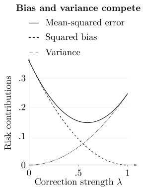
Exact finite-binomial risk for the specified state and sample count. The minimum lies near $\lambda=.594$, with MSE about $.1463$. This is a pointwise comparison using the true expectation for analysis; the location of that minimum is not available to an estimator that does not know $\mu$.

The pointwise optimum $\lambda_\star=\mu^2/(\mu^2+V)$ depends on the unknown answer. Practical regularization therefore needs a stated prior, a worst-case criterion or separate training data, followed by an honest assessment of transfer. Choosing the best correction after looking at the final reference answer does not demonstrate a predictive method. Data-driven mitigation explicitly raises this training-distribution question (Lowe et al., 2021).

Clipping an estimate to $[-1,1]$ cannot increase its squared error for a target in that interval: projection onto the interval moves every out-of-range value closer to every allowed target. It can introduce bias, and it does not automatically preserve an interval’s confidence coverage. Regularization changes the estimator class, so it does not contradict a theorem restricted to unbiased estimators.

Distinguish necessary and sufficient sample counts

For a fixed unbiased estimator expressed as an average of independent $Z_i\in[-\Gamma,\Gamma]$, Hoeffding’s inequality gives the sufficient choice

$N\geq\frac{2\Gamma^2}{\epsilon^2}\log\frac2\delta$

for error at most $\epsilon$ except with probability $\delta$. At $\Gamma=2,\epsilon=.02,\delta=.05$, this gives $73778$ records. It is conservative and is not a lower bound on all estimators. With a known bias bound $B<\epsilon$, use $\epsilon-B$ for the deviation about the estimator’s mean; uncertain calibration needs its own probability statement.

Signed combinations also depend on allocation. With independent strata, weights $(1.5,-.5)$, unit per-shot variance and $20000$ total shots:

Allocation	Shots in the two strata	Variance
Equal	$(10000,10000)$	$.00025$
Minimum variance	$(15000,5000)$	$.00020$

The optimum follows from $n_j\propto|w_j|\sigma_j$. Shared calibration or measurement records create covariance, so the independent-stratum formula then needs modification. See probabilistic cancellation and extrapolation for their specific sampling designs.

Read a circuit-level lower bound with its assumptions

Takagi, Tajima and Gu (2023), Theorem 3, consider $M$ qubits with local depolarization of strength at least $\gamma$ on every qubit after each of $L$ selected unitary layers. Intermediate operations are unital maps on those same $M$ qubits; a final arbitrary joint process receives $N$ distorted output states. This excludes encoded error correction from that circuit model.

Require absolute estimation error at most $\delta$ with probability at least $1-\varepsilon$ for every target state and observable. If two target expectations differ by more than $2\delta$, their bound implies

$N\geq\frac{(1-2\varepsilon)^2}{2\ln(2)\,M(1-\gamma)^{2L}}.$

For $M=4,L=200,\gamma=.02,\varepsilon=.05$, the right side is about $472.21$, requiring at least $473$ output states. For example, $|0000\rangle,|1111\rangle$ and observable $|0000\rangle\langle0000|$ are separated by one, so $\delta=.2$ meets the separation condition. The count is necessary, not sufficient; it excludes calibration costs and elapsed time.

The exponential dependence is on the selected noisy depth under these hypotheses. It is not a measured cost prediction for every device. Other results use different estimator classes: Tsubouchi, Sagawa and Yoshioka (2023) obtain quantum-estimation bounds for unbiased observable estimation in their virtual-circuit model, including depth scaling and width scaling for specified random-circuit ensembles. Those are distinct statements.

Quek et al. (2024) construct worst-case rapidly mixing circuit families with much stronger sampling barriers, allowing collective output measurements. Input-state knowledge matters: their input-aware result admits a classical-computation alternative. Their shortest-depth constructions and geometrically local variants have different connectivity assumptions. A particular finite experiment must match the relevant model before a bound can be applied.

These theorems constrain uniform promises over a family. A local observable with a small relevant region, a shallow circuit, or a restricted input family may remain tractable. Conversely, a few successful sizes do not determine the asymptotic scaling law. An expectation estimate does not establish accurate distribution sampling, state recovery or fault-tolerant computation.

Compare the complete experiment

Count calibration, circuit selection, modified runs, rejected outcomes and reference calculations along with science shots. Reusing calibration across many circuits can reduce its cost per answer, but only over a range where that calibration remains applicable. Test the combined estimator when methods share records or change the physical circuits; component variances and improvements do not simply add.

For independent acceptance probability $.18$, collecting $5000$ retained records needs $5000/.18\simeq27778$ attempts on average. Adding $6000$ calibration attempts and taking $1.4\,\mathrm{ms}$ per attempt gives expected time about $47.29\,\mathrm{s}$. A fixed budget near that mean does not guarantee $5000$ successes; a high-confidence budget requires a tail calculation. If the accepted mean is $.72$, the unnormalized moment is $.1296$. Neither equals the original ideal target without a physical argument; see symmetry verification.

Choose accuracy, confidence and cost measures that match the application. Compare with the raw estimator and an appropriate classical method on fresh tasks, including failures and uncertain reference values. If an unstable direction dominates, reducing correction strength or changing the experiment may help. If the application needs a long-lived unknown quantum state, estimation of a few final observables cannot supply it; quantum error correction addresses a different requirement.

Exercises

1. Prove the erasure limit

For the dephased $|+\rangle,|-\rangle$ example, show that every estimator has worst-case MSE at least one when it has no input label or other distinguishing information.

Solution

Its output $W$ has the same distribution under both inputs. Averaging the two risks gives $\tfrac12\mathbb E[(W-1)^2+(W+1)^2]=\mathbb E[W^2]+1\geq1$. At least one risk is therefore at least one. Returning zero attains this minimax value. Additional copies remain identically distributed, so they cannot lower it.

2. Derive the binary Fisher information

Compute the score of $p_x=(1+x\eta\mu)/2$ and show that the rescaled mean attains the unbiased variance bound.

Solution

The score is $x\eta/(1+x\eta\mu)$. Averaging its square gives $I=\eta^2/(1-\eta^2\mu^2)$. Since $\operatorname{Var}(X)=1-\eta^2\mu^2$, the estimator $\overline X/\eta$ has variance $1/(NI)$. This uses known attenuation, independent records and interior parameters; it does not prohibit lower pointwise MSE with bias.

3. Find the pointwise shrinkage minimum

Differentiate the plotted risk and explain why its minimizer is not immediately an implementable prescription.

Solution

Setting $-2(1-\lambda)\mu^2+2\lambda V=0$ gives $\lambda_\star=\mu^2/(\mu^2+V)$. Here $V=.2464$, hence $\lambda_\star\simeq.5937$ and minimum risk $\mu^2V/(\mu^2+V)\simeq.1463$. Both depend on the unknown $\mu$. An estimator needs a choice based on permitted information and a new risk analysis for any data-dependent tuning.

4. Check a clipping claim

Prove that clipping to $[-1,1]$ cannot increase squared error for $\mu\in[-1,1]$. Does this imply unbiasedness?

Solution

Values already inside the interval do not change. If $W>1$, then $0\leq1-\mu\leq W-\mu$; if $W<-1$, the analogous inequality holds at $-1$. Squaring proves the pointwise result and averaging proves the MSE result. The clipping transformation is nonlinear and need not preserve the estimator’s expectation.

5. Separate three meanings of a sample count

Classify the counts $568572$, $73778$ and $473$ above.

Solution

The first meets a specified standard error in an exactly solved binary attenuation model at $\mu=0$. The second is a sufficient concentration bound for independent bounded unbiased outputs. The third is a necessary circuit-model lower bound. They address different models and accuracy criteria, so their numerical ordering is not a comparison of competing protocols.

6. Distinguish expected and reliable acceptance budgets

Let each independent attempt succeed with probability $a$. Give the mean and variance of the attempt count needed for $m$ successes, and a fixed-budget expression for the chance of obtaining fewer than $m$.

Solution

The stopping count is a sum of $m$ independent geometric waiting times:

$$\begin{aligned} \mathbb E T&=m/a,\\ \operatorname{Var}(T)&=m(1-a)/a^2. \end{aligned}$$

With a fixed $N$ attempts, the failure probability is $\sum_{k=0}^{m-1}\binom Nk a^k(1-a)^{N-k}$. The expectation $m/a$ is not a high-confidence budget. For $a=.18,m=5000$, the stopping-time standard deviation is about $356$ attempts.

References

• A. Lowe, M. H. Gordon, P. Czarnik, A. Arrasmith, P. J. Coles, and L. Cincio, “Unified Approach to Data-Driven Quantum Error Mitigation,” Physical Review Research 3, 033098 (2021), doi:10.1103/PhysRevResearch.3.033098.
• Y. Quek, D. Stilck França, S. Khatri, J. J. Meyer, and J. Eisert, “Exponentially Tighter Bounds on Limitations of Quantum Error Mitigation,” Nature Physics 20, 1648–1658 (2024), doi:10.1038/s41567-024-02536-7.
• R. Takagi, S. Endo, S. Minagawa, and M. Gu, “Fundamental Limits of Quantum Error Mitigation,” npj Quantum Information 8, 114 (2022), doi:10.1038/s41534-022-00618-z.
• R. Takagi, H. Tajima, and M. Gu, “Universal Sampling Lower Bounds for Quantum Error Mitigation,” Physical Review Letters 131, 210602 (2023), doi:10.1103/PhysRevLett.131.210602.
• K. Tsubouchi, T. Sagawa, and N. Yoshioka, “Universal Cost Bound of Quantum Error Mitigation Based on Quantum Estimation Theory,” Physical Review Letters 131, 210601 (2023), doi:10.1103/PhysRevLett.131.210601.