Measurement Error Mitigation

Measurement-error mitigation uses a calibrated detector response to estimate the probabilities or observables that an ideal terminal measurement would have produced. The key question is an inverse problem: which latent distributions could have generated the recorded outcomes, and how uncertain is the inferred answer?

This page develops response-matrix inversion, constrained fitting and observable-specific correction. It separates errors from finite sampling, uncertain calibration and an incorrect detector model. The correction estimates terminal statistics; it does not undo measurement backaction or repair an earlier feedforward operation.

Helpful background. SPAM errors explains when detector response can be separated from preparation and coherence effects. Error mitigation introduces bias, variance and sampling cost. Variance and covariance supplies uncertainty propagation.

The classical detector-response model

Let $p_z$ be the probability of ideal outcome $z$, and let $q_y$ be the probability of reported outcome $y$. The response model is

$$\begin{aligned} A_{y|z}&=\Pr(y\text{ reported}\mid z\text{ ideal}),\\ q_y&=\sum_zA_{y|z}p_z,\\ \sum_yA_{y|z}&=1,\qquad A_{y|z}\geq0. \end{aligned}$$

Reported outcomes label rows; ideal outcomes label columns. Thus $\mathbf q=A\mathbf p$, with each column normalized. All report types—including a resolved erasure or invalid classifier output—must be counted or deliberately merged. Silently discarding reports changes the probabilities being modeled.

For a computational-basis measurement, this relation holds for every input state precisely when its POVM effects have the form

$M_y=\sum_zA_{y|z}|z\rangle\langle z|.$

Under that assumption, $A$ determines the diagonal POVM. It still does not determine the state after measurement. Basis calibration alone measures the diagonal matrix elements and cannot exclude off-diagonal effects. The more limited relation may also hold on a specified family of input states without determining the detector on all states. See measurement tomography and Maciejewski, Zimborás and Oszmaniec (2020).

Calibration also assumes sufficiently well-known input preparations. If commands prepare latent labels through a response $B$, the measured command-to-report table is $C=AB$. Only trusted basis preparations, $B=I$, make $C=A$ directly. A separately known full-row-rank $B$ can also identify $A$; otherwise the factorization may be ambiguous. More repeated commands cannot by themselves resolve this ambiguity.

A binary detector, step by step

Write

$$\begin{aligned} A&=\begin{pmatrix}1-\alpha&\beta\\\alpha&1-\beta\end{pmatrix},\\ d&=1-\alpha-\beta. \end{aligned}$$

Here $\alpha$ is the probability of reporting one for ideal zero, and $\beta$ is the reverse error. Since $p_1=1-p_0$,

$$\begin{aligned} q_0&=\beta+dp_0,\\ p_0&=(q_0-\beta)/d\quad(d\ne0). \end{aligned}$$

For the signed moment $m=p_0-p_1$, let $m_{\rm obs}=q_0-q_1$. Then

$$\begin{aligned} m_{\rm obs}&=(\beta-\alpha)+dm,\\ m&=\frac{m_{\rm obs}-(\beta-\alpha)}{d}. \end{aligned}$$

The offset matters when the errors are asymmetric. If $d=0$, the two response columns coincide and all latent distributions give the same reports. If $d<0$, the detector is more often reversed than correct, but remains algebraically invertible. Sensitivity grows as $|d|$ approaches zero.

For $\alpha=.08$, $\beta=.18$ and $\mathbf p=(.35,.65)^{\mathsf T}$, the reports are $(.439,.561)^{\mathsf T}$. The raw signed mean is $-.122$, while correction gives the intended $-.3$. This corrects detector bias under the model; it does not subtract errors in the prepared state itself.

Identifiability and sensitivity

Full-distribution recovery on the unrestricted probability simplex requires full column rank of $A$. If $A\mathbf v=0$, column stochasticity implies $\mathbf1^{\mathsf T}\mathbf v=0$. Small positive and negative displacements along $\mathbf v$ therefore produce different interior distributions with identical reports. Additional data can narrow sampling uncertainty without distinguishing them.

For square nonsingular $A$, the linear estimate is $\widehat{\mathbf p}=A^{-1}\widehat{\mathbf q}$. A tall full-column-rank response also has a left inverse and can recover the full distribution; it need not lose information just because it is rectangular. For deficient rank, a pseudoinverse chooses a projection, not the missing probabilities.

Singular values describe sensitivity. A perturbation along a left singular vector with singular value $s$ is amplified by $1/s$ in inversion. Small singular values can amplify science-shot fluctuations, calibration errors and model mismatch. A condition number is not a test of the model: even the identity is perfectly conditioned while being a completely wrong description of a particular detector.

Negative estimates can be ordinary sampling fluctuations

Consider the correctly known response

$A=\begin{pmatrix}.6&.4\\.4&.6\end{pmatrix}.$

Every physical latent distribution gives $q_0\in[.4,.6]$. If empirical frequencies are $(.35,.65)$, inversion yields $(-.25,1.25)$. These are signed statistical estimates, not physical negative probabilities.

Crucially, empirical frequencies need not lie inside the forward image of the simplex. When the true $p_0=0$, one has $q_0=.4$, yet with $20$ independent shots the probability of observing $\widehat q_0\leq.35$ is about $.415893$. With $1000$ shots that lower-tail probability is about $.000645$. A residual must be compared with its sampling distribution and calibration uncertainty before interpreting it as model failure.

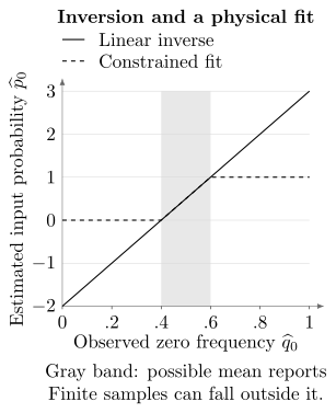
For the response above, inversion gives $\widehat p_0=5\widehat q_0-2$. Binary constrained least squares and multinomial maximum likelihood clip that value into $[0,1]$. The gray strip marks the possible mean reported probabilities; finite samples can fall outside it. The constrained estimate remains physical but generally acquires boundary bias.

Fitting a physical distribution

For a probability vector $\mathbf p$, constrained least squares minimizes a weighted forward residual. Multinomial maximum likelihood instead maximizes the likelihood of the counts:

$$\begin{aligned} \widehat{\mathbf p}_{\rm LS} &=\underset{\mathbf p\in\Delta}{\operatorname{arg\,min}} \,L(\mathbf p),\\ L(\mathbf p)&=(\widehat{\mathbf q}-A\mathbf p)^{\mathsf T} W(\widehat{\mathbf q}-A\mathbf p),\\ \widehat{\mathbf p}_{\rm ML} &=\underset{\mathbf p\in\Delta}{\operatorname{arg\,max}} \,\sum_y n_y\log(A\mathbf p)_y, \end{aligned}$$

where $\Delta$ is the normalized nonnegative simplex and $W$ is a chosen positive weight matrix. A zero count contributes zero to the likelihood; a positive count at zero modeled probability makes the log likelihood $-\infty$.

For the preceding binary example, both methods choose $(0,1)$ and predict $(.4,.6)$ when the observed frequencies are $(.35,.65)$. Their agreement is special to this one-parameter case; in larger problems the objectives can give different answers. Physical output alone does not prove that the response is correct. Constraints and regularization can reduce variance at the price of bias, especially near a boundary.

Iterative unfolding

Iterative Bayesian unfolding is a multiplicative update (D’Agostini, 1995; Nachman et al., 2020):

$$\begin{aligned} q_y^{(k)}&=\sum_zA_{y|z}p_z^{(k)},\\ p_z^{(k+1)}&=p_z^{(k)}\sum_y A_{y|z}\frac{\widehat q_y}{q_y^{(k)}}. \end{aligned}$$

One way to understand it is to assign each reported count fractionally to possible latent labels using the current conditional probabilities $A_{y|z}p_z^{(k)}/q_y^{(k)}$, then add these assigned counts. Summing over $z$ proves normalization. The denominator must be positive wherever $\widehat q_y>0$; a zero-count, zero-prediction row contributes zero. Start with positive mass on every latent outcome that may be needed, because the update cannot revive a zero component.

This is also an expectation–maximization update for the fixed-response mixture likelihood. Exact updates do not decrease that likelihood, but a stopped iterate depends on its initialization and stopping rule. It is not automatically a posterior distribution over the unknown probabilities. Early stopping acts as regularization; choosing its stopping point from the final comparison data can bias the comparison.

For the binary example, starting from $(.5,.5)$ gives $(.47,.53)$ after one step and approximately $(.441300,.558700)$ after two. The sequence approaches the likelihood boundary. The remaining forward discrepancy still needs a statistical interpretation.

Estimate an observable without reconstructing every probability

For a diagonal target with values $f_z$, the desired mean is $\mu=\mathbf f^{\mathsf T}\mathbf p$. Find report-dependent weights satisfying

$A^{\mathsf T}\mathbf w=\mathbf f.$

Then the average of the observed weights is unbiased under a known correct response:

$$\begin{aligned} \widehat\mu&=\frac1N\sum_{j=1}^Nw_{Y_j},\\ \mathbb E\widehat\mu&=\mathbf w^{\mathsf T}A\mathbf p=\mu. \end{aligned}$$

The equation is solvable precisely when $\mathbf f$ lies in the row space of $A$. On the unrestricted simplex this is also the condition for the observable to be identifiable: an unobservable null direction must not change the target. For example, a detector that distinguishes label two from labels zero and one together identifies their total population, although it cannot distinguish zero from one.

For the asymmetric binary example and $\mathbf f=(1,-1)^{\mathsf T}$,

$\mathbf w=(45/37,-55/37)^{\mathsf T}.$

Average $45/37$ for each reported zero and $-55/37$ for each reported one. The weights need not lie in the observable’s physical range. Their fluctuations determine the sampling cost.

For independent reports and fixed weights,

$$\begin{aligned} \operatorname{Cov}(\widehat{\mathbf q}) &=\frac{\operatorname{diag}(\mathbf q)-\mathbf q\mathbf q^{\mathsf T}}{N},\\ \operatorname{Var}(\widehat\mu) &=\frac{\sum_yq_yw_y^2-\mu^2}{N}. \end{aligned}$$

With $N=1000$, the binary example gives variance approximately $.001799$. When weights are nonunique, a minimum-Euclidean-norm choice need not minimize variance. A reference distribution can instead guide variance minimization, but weights fitted using science data require analysis of that extra dependence. For designed randomized expectation estimators, see van den Berg, Minev and Temme (2022).

Include calibration uncertainty

Each calibrated column is a multinomial estimate. With $M_z$ independent trusted preparations of $z$, its covariance is

$$\operatorname{Cov}(\widehat{\mathbf A}_{\cdot|z}) =\frac{\operatorname{diag}(\mathbf A_{\cdot|z}) -\mathbf A_{\cdot|z}\mathbf A_{\cdot|z}^{\mathsf T}}{M_z}.$$

Fitting a response and then treating it as exactly known omits this uncertainty. Independent column calibrations give independent sampling errors only if they share no fluctuating nuisance parameters or records.

For the binary signed moment, local derivatives at the true parameters are

$$\begin{aligned} \frac{\partial m}{\partial q_0}&=\frac2d,\\ \frac{\partial m}{\partial\alpha}&=\frac{2p_0}{d},\\ \frac{\partial m}{\partial\beta}&=-\frac{2(1-p_0)}d. \end{aligned}$$

Use $1000$ science shots and $100$ calibration shots for each column of the asymmetric detector. Propagating the three independent binomial variances gives the following rounded delta-method results:

Contribution	Variance
Science sampling	$.001799$
Detector calibration	$.005214$
Sum	$.007013$

The corresponding standard error is about $.083742$. These are local approximations for a fitted inverse, not exact unbiased-ratio guarantees. They become unreliable near singular response matrices, low counts or active constraints. Joint likelihood, resampling of the complete calibration-and-science procedure, and coverage simulations are useful alternatives, with their own assumptions.

If two corrected values reuse calibration parameters $\theta$, their leading shared covariance is $\mathbf g_i^{\mathsf T}\operatorname{Cov}(\widehat\theta)\mathbf g_j$, where $\mathbf g_i$ is the correction’s sensitivity to $\theta$. More science shots do not eliminate that shared component. Include cross terms as well if science and calibration acquisitions are dependent.

Drift causes a different error. If the live detector changes to $\alpha=.12,\beta=.22$ at the same $p_0=.35$, it gives $q_0=.451$. The old correction reports $m\simeq-.267568$, a bias of $.032432$. That shift does not disappear with more science samples. Interleaved known probes, context-matched checks and time-resolved residuals can reveal it.

Multiqubit structure and randomized readout

An unrestricted $n$-bit response has $2^n(2^n-1)$ free parameters. A product model $A=\bigotimes_jA^{(j)}$ has only $2n$, but assumes each reported bit depends only on its own ideal bit and that reports are conditionally independent. That assumption needs joint tests.

For ideal $00$, compare a pair-flip detector with independent flips of probability $.1$:

Reports in order $00,01,10,11$	Probability vector
Pair flips	$(.9,0,0,.1)$
Independent flips	$(.81,.09,.09,.01)$

The one-bit error rates agree, but the total-variation distance is $.18$ and the pair-flip covariance is $.09$. Their parity responses differ strongly. Bravyi et al. (2021) develop product and correlated-response methods. Cluster models retain selected correlations; their omitted interactions remain an assumption. Matrix-free and observed-support approaches can reduce computation (Nation et al., 2021), but an unrestricted detector does not become identifiable from fewer calibration data merely because its inverse is never stored.

What bit-flip averaging removes

Apply an ideal randomly chosen bit mask $s$ before readout and undo the mask in the report. For a fixed classical response, uniform averaging gives

$\widetilde A_{y|z}=2^{-n}\sum_sA_{y\oplus s|z\oplus s}.$

It now depends only on the flip pattern $y\oplus z$. There are $2^n-1$ independent pattern probabilities, and an ideal zero-string calibration with the same randomized protocol can sample that pattern distribution. Resolving a general distribution still costs samples; correlations remain (Smith et al., 2021).

For one bit, the asymmetric example becomes

$\widetilde A=\begin{pmatrix}.87&.13\\.13&.87\end{pmatrix}.$

The offsets have been symmetrized. The inserted controls must work as modeled and must not change readout through unaccounted context dependence. Moreover, random $X$ masks alone do not generally eliminate off-diagonal POVM effects; the classical-response assumption still matters. Exercise 6 gives a counterexample. More elaborate randomized protocols can have different assumptions.

Erasures, feedforward and meaningful comparisons

A tall response can include erasure reports. For

$A=\begin{pmatrix}.9&.1\\.05&.7\\.05&.2\end{pmatrix},$

the input $\mathbf p=(.6,.4)^{\mathsf T}$ gives reports $(.58,.31,.11)^{\mathsf T}$. Discarding the third outcome leaves acceptance $.89$ and conditional reports $(58/89,31/89)$, not the original populations. Keep acceptance and rejected attempts when comparing precision and cost. Unmodeled latent leakage requires additional input sectors or bounds; extra reported rows alone do not characterize it.

For an earlier measurement inside a circuit, a wrong report may already have selected the wrong gate or conditional state. Relabeling the final stored bit cannot reverse that physical action. Measurement in circuits and quantum instruments explain the conditional maps needed by a causal correction protocol.

A useful comparison checks both the assumed response and the complete estimator. Test representative joint outcomes and coherent probes where needed; account for sampling when interpreting residuals; and compare corrected and raw results at equal total resources. Calibration reuse saves cost only while its response remains applicable. Choose model complexity, regularization and stopping with data separate from the final performance comparison. These steps distinguish a successful inference from an accidentally favorable estimate.

Exercises

1. Separate preparation and detector response

Use the asymmetric detector above, $B=((.95,.10),(.05,.90))$, and $\mathbf p=(.35,.65)^{\mathsf T}$. Compare corrections using $A$ and the empirical command-to-report table $C=AB$.

Solution

One finds

$C=\begin{pmatrix}.883&.254\\.117&.746\end{pmatrix}.$

The reports are $(.439,.561)^{\mathsf T}$. Inverting $A$ recovers $(.35,.65)$; inverting $C$ gives $(5/17,12/17)$ instead. The second inverse has included preparation error in the detector model. Directly identifying $C=A$ requires trusted matching basis preparations, or a separate argument establishing the relevant factorization.

2. Derive the binary inverse and its variance

Find $A^{-1}$ and the report weights for the signed observable. Recover the science-shot variance in the worked example.

Solution

For $d\ne0$,

$A^{-1}=\frac1d\begin{pmatrix}1-\beta&-\beta\\-\alpha&1-\alpha\end{pmatrix}.$

Multiplication by the row $(1,-1)$ gives the two weights. In the example they are $45/37$ and $-55/37$, so the variance is $(100/37)^2q_0(1-q_0)/N\simeq.001799$ for $N=1000$. At $d=0$, the columns coincide; no unbiased weighting recovers the signed moment on every input.

3. Explain a negative inverse without rejecting the model

For the symmetric $.6/.4$ response, observe seven zero reports in $20$ shots. Compute the inverse, constrained fit and first two unfolding iterates from a uniform start. Is this observation enough to reject the response?

Solution

The inverse is $(-.25,1.25)$; the constrained least-squares and likelihood estimates are $(0,1)$. Unfolding gives $(.47,.53)$ and approximately $(.441300,.558700)$. If the true $p_0=0$, then

$\Pr(K\leq7)=\sum_{k=0}^7\binom{20}{k}.4^k.6^{20-k}\simeq.415893.$

The downward fluctuation is common under a member of the assumed family. A negative inverse is therefore not, by itself, a statistically significant rejection. The uncertainty of calibration and any selection of which residual to inspect must also be considered.

4. Identify a target when the distribution is not identifiable

Let $A=((1,1,0),(0,0,1))$. Which of $f=(1,1,-1)$ and $g=(1,-1,0)$ can be recovered on every input distribution?

Solution

For $f$, choose report weights $w=(1,-1)$; then $A^{\mathsf T}w=f$. For $g$, the first two components of $A^{\mathsf T}w$ are always equal, so no solution exists. The latent distributions $(1,0,0)$ and $(0,1,0)$ have identical reports but opposite $g$ values. Additional reports do not remove this ambiguity.

5. Detect correlations invisible in marginal errors

For the pair-flip and independent-flip distributions in the table, calculate total variation, connected flip covariance and parity expectation.

Solution

Total variation is half the sum of four absolute differences, giving $.18$. The pair model has $\mathbb E(F_1F_2)=.1$ and marginal means $.1$, so covariance is $.09$; the independent model has covariance zero. For parity $(-1)^{Y_1+Y_2}$, the respective means are $1$ and $.64$. Matching one-bit error rates does not determine the correction of parity.

6. Test the scope of bit-flip averaging

First symmetrize the asymmetric classical detector. Then consider a qubit POVM with $M_0=I/2+.2Y+.3Z$ and $M_1=I-M_0$. Does randomly applying $X$ and undoing it in the reported bit make this second measurement diagonal?

Solution

The classical average is $(A+XAX)/2$, giving diagonal entries $.87$ and off-diagonal entries $.13$. In the POVM example,

$\widetilde M_0=\tfrac12(M_0+XM_1X)=M_0.$

It is a valid effect because its eigenvalues are $1/2\pm\sqrt{.13}$. Its $Y$ component survives. Basis inputs would suggest columns with zero-report probabilities $.8$ and $.2$, predicting $.5$ for $|+y\rangle$ from its populations, whereas the actual probability is $.7$. The classical averaging formula cannot be extended to every coherent detector merely from basis calibration.

7. Propagate finite calibration and drift

Reproduce the uncertainty table using independent binomial science and calibration data. Explain why repeated science shots cannot cure the stale-response bias.

Solution

Use variances $q_0(1-q_0)/1000$, $\alpha(1-\alpha)/100$ and $\beta(1-\beta)/100$ with the three derivatives in the text. Science contributes about $.001799$ and calibration $.005214$, giving $.007013$ in total. These are delta-method values. A shared calibration contributes cross-covariance to multiple corrected estimates. Drift to $(.12,.22)$ moves the mean report to $.451$ and the stale corrected moment to $-.267568$; its bias persists as the number of science shots tends to infinity.

8. Recover populations with an erasure report

Use the three-row response in the text. Show that all reports can identify the two input populations, while simply conditioning on the first two reports gives a different distribution.

Solution

The columns are linearly independent, so a left inverse recovers $\mathbf p$ from the full reported vector under this model. Here $q_0=.1+.8p_0$, hence $p_0=(.58-.1)/.8=.6$. Conditioning alone gives $(58/89,31/89)$, approximately $(.651685,.348315)$. It includes detector misassignment and state-dependent erasure; it is not the corrected latent distribution. In a mid-circuit experiment these report probabilities also do not specify the surviving conditional states.

References

• S. Bravyi, S. Sheldon, A. Kandala, D. C. McKay, and J. M. Gambetta, “Mitigating measurement errors in multiqubit experiments,” Physical Review A 103, 042605 (2021), doi:10.1103/PhysRevA.103.042605.
• G. D’Agostini, “A multidimensional unfolding method based on Bayes’ theorem,” Nuclear Instruments and Methods in Physics Research A 362, 487–498 (1995), doi:10.1016/0168-9002(95)00274-X.
• F. B. Maciejewski, Z. Zimborás, and M. Oszmaniec, “Mitigation of readout noise in near-term quantum devices by classical post-processing based on detector tomography,” Quantum 4, 257 (2020), doi:10.22331/q-2020-04-24-257.
• B. Nachman, M. Urbanek, W. A. de Jong, and C. W. Bauer, “Unfolding quantum computer readout noise,” npj Quantum Information 6, 84 (2020), doi:10.1038/s41534-020-00309-7.
• P. D. Nation, H. Kang, N. Sundaresan, and J. M. Gambetta, “Scalable mitigation of measurement errors on quantum computers,” PRX Quantum 2, 040326 (2021), doi:10.1103/PRXQuantum.2.040326.
• A. W. R. Smith, K. E. Khosla, C. N. Self, and M. S. Kim, “Qubit readout error mitigation with bit-flip averaging,” Science Advances 7, eabi8009 (2021), doi:10.1126/sciadv.abi8009.
• E. van den Berg, Z. K. Minev, and K. Temme, “Model-free readout-error mitigation for quantum expectation values,” Physical Review A 105, 032620 (2022), doi:10.1103/PhysRevA.105.032620.