Zero-Noise Extrapolation

Zero-noise extrapolation estimates an ideal expectation by repeating a computation with deliberately increased noise and extrapolating back toward zero noise. Its central tradeoff is simple: cancellation can reduce systematic error, but the signed combination of measurements amplifies statistical fluctuations. A good extrapolation needs both a physically meaningful noise-scaling experiment and a defensible statistical model.

The zero of the scaled noise coordinate need not remove every error. Preparation, readout, unscaled gates and approximation errors can remain. Throughout this page, the intended endpoint is stated separately from the fully ideal answer.

Required background. Error mitigation explains bias, variance and total sampling cost. Markovian and non-Markovian noise explains why repeating an operation need not multiply a fixed noise generator.

Helpful background. Variance and covariance supplies uncertainty propagation. Circuit model fixes ideal composition and inverse operations.

The noise coordinate and its zero limit

For input $\rho$, ideal circuit channel $\mathcal U$ and observable $O$, define

$\mu_{\rm id}=\operatorname{Tr}[O\mathcal U(\rho)].$

Write the actual experimental family as $\widetilde{\mathcal C}_{c\epsilon,\eta}$, where $\epsilon$ is a baseline noise strength, $c\geq1$ is its gain, and $\eta$ denotes unscaled background effects. Its mean is

$$\begin{aligned} \mu(c;\eta)&=\operatorname{Tr}[O\widetilde{\mathcal C}_{c\epsilon,\eta}(\rho)],\\ \mu_{0|\eta}&=\mu(0;\eta). \end{aligned}$$

The device supplies data at $c\geq1$. Extrapolation estimates the unexecuted endpoint $\mu_{0|\eta}$. It equals $\mu_{\rm id}$ only if the remaining effects are absent or otherwise accounted for. For example, if readout reports $a+b\mu(c)$, extrapolating gate noise leaves $a+b\mu_{0|\eta}$, including the detector’s offset and contrast.

Temme, Bravyi and Gambetta (2017), and Li and Benjamin (2017), developed noise extrapolation for quantum computations. Its perturbative starting point is

$$\mu(c;\eta)=\mu_{0|\eta} +\sum_{k=1}^{p}a_k(c\epsilon)^k+R_{p+1}(c\epsilon).$$

The same coefficients must describe all chosen gains, and the remainder must be controlled throughout that range. Smooth-looking data alone do not establish either assumption. Time-correlated noise is not automatically fatal, but stretching or folding can change its spectrum rather than multiply its strength (Schultz et al., 2022).

Cancel low-order terms with Richardson extrapolation

Choose $p+1$ distinct gains and combine their sample means:

$\widehat\mu_R=\sum_{i=0}^{p}w_i\widehat\mu(c_i).$

Substituting the expansion shows exactly what the weights must do:

$$\begin{aligned} \sum_iw_i&=1,\\ \sum_iw_i c_i^k&=0\qquad(1\leq k\leq p). \end{aligned}$$

The first condition preserves the constant term. The others cancel the first $p$ powers of noise. Evaluating the Lagrange interpolation polynomial at zero gives

$w_i=\prod_{j\ne i}\frac{c_j}{c_j-c_i}.$

For gains $(1,2,3)$, $w=(3,-3,1)$: the zeroth, first, second and third weighted moments are $(1,0,0,6)$. Thus a controlled cubic contribution survives as $6a_3\epsilon^3$. More generally,

$\sum_iw_i c_i^{p+1}=(-1)^p\prod_i c_i.$

This identity specifies a leading term, not a bound on an unknown remainder. For the illustrative curve

$$\begin{aligned} \mu(c)&=.42-.30x+.18x^2-.07x^3,\\ x&=.04c, \end{aligned}$$

the three means are approximately $.408284$, $.397116$ and $.386471$. Their combination is $.41997312$: the exact bias for this cubic is $-2.688\times10^{-5}$.

Why the result can be much noisier

At two gains $(1,s)$, with $s>1$,

$$\begin{aligned} \widehat\mu_R&=\frac{s\widehat\mu(1)-\widehat\mu(s)}{s-1},\\ \Lambda&=\sum_i|w_i|=\frac{s+1}{s-1}. \end{aligned}$$

Nearby gains make the denominator small, magnifying fluctuations and gain errors. Widely separated gains reduce this coefficient norm but probe farther from the weak-noise limit. Larger gain is therefore not always better. Krebsbach, Trauzettel and Calzona (2022) analyze this competition in Richardson designs.

An extrapolate can lie outside the spectral range of $O$ because its weights are signed. It is an estimator, not the expectation of a reconstructed physical state. Clipping it changes the estimator and generally introduces bias; a bounded statistical model needs its own uncertainty analysis.

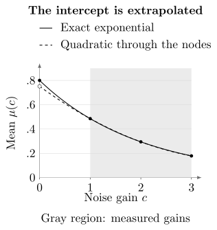
An exact mean $\mu(c)=.8e^{-.5c}$ and its quadratic interpolant agree at $c=1,2,3$, but the extrapolated intercept is about $.7513$ rather than $.8$. These are exact node means: the discrepancy is model truncation, even before sampling uncertainty. The gray region contains the three measured gains.

How physical noise can be amplified

Folding a unitary circuit

Global unitary folding replaces

$U\longmapsto U(U^\dagger U)^n.$

The ideal product remains $U$ and its nominal depth factor is $2n+1$. Local folding inserts inverse pairs around selected gates or layers; partial folding averages over subsets to obtain intermediate nominal factors (Giurgica-Tiron et al., 2020). Inspect the final native circuit, since a compiler may remove the inserted pairs or change routing.

Depth is not automatically noise gain. If the erroneous forward gate is $G_\epsilon$ and the erroneous inverse is exactly $G_\epsilon^\dagger$, then the physical fold gives $G_\epsilon G_\epsilon^\dagger G_\epsilon=G_\epsilon$: its coherent error has not increased at all. Other inverse implementations can amplify or rotate different errors. Gate count, leakage, crosstalk and idle time need not scale together.

Repeated shots on one randomly selected fold pattern also do not estimate variation between patterns. Use multiple instances when the protocol averages over them.

Stretching a pulse

If the full noiseless Hamiltonian $K(t)$ acts for duration $T$, then

$K_c(t)=K(t/c)/c,\qquad 0\leq t\leq cT$

produces the same time-ordered ideal unitary. The substitution $u=t/c$ shows why. Under a fixed, control-independent dissipative generator $\mathcal L$, the master equation in $u$ becomes

$\frac{d\rho}{du}=-\frac{i}{\hbar}[K(u),\rho]+c\mathcal L(\rho).$

This gives an exact noise-strength rescaling within that model, even when the Hamiltonian and dissipator do not commute. Stretching only the driven part while leaving a drift Hamiltonian unscaled need not preserve the target. Drive-dependent noise, bandwidth distortion and colored noise can also invalidate this simple equation.

Adding a randomized Pauli channel

For a characterized Pauli–Lindblad noise layer,

$$\mathcal E=e^{\mathcal L},\qquad \mathcal L=\sum_j\lambda_j(\mathcal P_j-\mathcal I),$$

where $\mathcal P_j(\rho)=P_j\rho P_j$ and $\lambda_j\geq0$, add the physical channel $e^{(G-1)\mathcal L}$ at the appropriate layer boundary. The combined modeled noise is $e^{G\mathcal L}$, $G\geq1$. Each added Pauli has probability

$p_j(G)=\frac{1-e^{-2(G-1)\lambda_j}}2.$

Pauli conjugation superoperators commute, even for anticommuting Pauli operators, so the elementary channels can be composed in any order. Individual randomized circuits need not implement the noiseless circuit; it is their specified ensemble that realizes the amplified channel. Negative fitted rates do not define these physical probabilities. The model, inserted controls and layer placement must apply to the actual experiment (Mari, Shammah and Zeng, 2021).

Requested gain versus effective gain

Suppose nominal gains $(1,2,3)$ are actually $(1,1.9,3.2)$. The nominal weights give the first moment $3-3(1.9)+3.2=.5$, so the supposedly canceled linear term returns as $.5a_1\epsilon$.

For the earlier cubic and actual gains $(1,1.8,2.55)$, recalibration changes the comparison:

Quantity	Nominal weights	Calibrated weights
Weights	$(3,-3,1)$	$(3.702,-4.25,1.548)$
Estimate	$.41813$	$.41998$
Absolute-weight sum	$7$	$9.5$

The calibrated estimate is less biased here but more sensitive to sampling. A scalar gain may still be inadequate if different error mechanisms respond differently. Interleave gains in time and repeat baseline circuits to distinguish gain dependence from drift; use diagnostics matched to the gates and observables of interest.

Sampling, covariance and fitting

For independent node means with per-shot variances $\sigma_i^2$ and $N_i$ shots,

$\operatorname{Var}(\widehat\mu_R)=\sum_i\frac{w_i^2\sigma_i^2}{N_i}.$

Minimizing this variance with a fixed total $N$ gives

$$\begin{aligned} N_i&=N\frac{|w_i|\sigma_i}{\sum_j|w_j|\sigma_j},\\ \operatorname{Var}_{\min}&=\frac{(\sum_i|w_i|\sigma_i)^2}{N}. \end{aligned}$$

For equal per-shot variances this produces a relative factor $\Lambda^2$ compared with one raw mean at the same shot budget. It is not a universal cost formula. If each attempt takes time $\tau_i$, fixed-time allocation instead satisfies $N_i\propto |w_i|\sigma_i/\sqrt{\tau_i}$. Include calibration, longer circuits, random instances and rejected attempts in resource comparisons.

With $w=(3,-3,1)$, $\sigma=(.6,.8,.5)$ and $N=47000$, the optimal allocation is $(18000,24000,5000)$ and the variance is $.000470$. Equal allocation gives about $.0005904$.

If node estimates share calibration or drift, use their full covariance $\Sigma$:

$\operatorname{Var}(\widehat\mu_R)=w^{\mathsf T}\Sigma w.$

For the preceding allocation, adding the same random offset of variance $.000002$ to every node makes the result $.000472$. Dropping its cross-covariances instead gives $.000508$. An identical additive offset survives because $\sum_iw_i=1$; other shared patterns can increase or decrease uncertainty.

Calibrated gains are uncertain too. With $h(y,c)=w(c)^{\mathsf T}y$, combine the data and gain gradients into $g=\nabla h$. The leading propagated variance is $g^{\mathsf T}\operatorname{Cov}(y,c)g$, including cross terms. Near-coincident gains can make those derivatives large. Resampling must reproduce the acquisition’s calibration, instance and time dependence.

Fit more points than coefficients when possible

With design $X_{ik}=c_i^k$ and positive-definite covariance $\Sigma$, generalized least squares gives

$$\begin{aligned} B&=X^{\mathsf T}\Sigma^{-1}X,\\ \widehat\beta&=B^{-1}X^{\mathsf T}\Sigma^{-1}y. \end{aligned}$$

This requires full column rank; $\widehat\beta_0$ is the intercept. Exact interpolation through $p+1$ points has no residual degrees of freedom. Additional gains can test the model’s predictions, but do not themselves observe the interval from zero to baseline noise.

An exponential $a+be^{-\gamma c}$ needs a physical reason. With known $a$, two distinct nondegenerate means can identify $b,\gamma$ in the exact model; with unknown $a$, at least three suitable gains are needed. Flat data, $b=0$, coincident rates in multiexponential models and saturation can make inference unidentifiable or very unstable. Taking logarithms requires compatible signs and changes the statistical error model.

Choose model order, gain range and any constraints independently of the final performance comparison. Test intermediate gains, known-answer circuits and sensitivity to the range. A small fitting residual cannot prove the zero-noise endpoint: many smooth curves agree at finitely many nonzero nodes and disagree at zero.

Combining extrapolation with other corrections

A fixed affine readout correction $T(q)=Lq+b$ commutes with fixed Richardson weights because their sum is one. This remains an algebraic identity even for uncertain shared calibration, but its covariance must still be propagated. Gain-dependent calibration, clipping and constrained fitting generally break the equivalence. See measurement-error mitigation.

Conditioning on a symmetry gives a ratio of a projected numerator and an acceptance probability. Extrapolating the two separately and then dividing is generally different from extrapolating their ratio. Rejected attempts and gain-dependent acceptance remain part of the cost and uncertainty. Symmetry verification develops that distinction.

For several independently varied noise coordinates, total-degree-$d$ polynomials in $\ell$ variables have $\binom{d+\ell}{d}$ coefficients. That many nodes are necessary to determine the whole polynomial, and full rank is still required. Fewer nodes can sometimes determine the intercept along a constrained path; they cannot generally identify every coefficient. Scaling only selected coordinates leaves the others at the extrapolated endpoint.

Exercises

1. Change the Richardson nodes

Find quadratic-cancellation weights for $(1,2,4)$ and the first uncanceled moment.

Solution

The weights are $(8/3,-2,1/3)$. Their moments through degree three are $(1,0,0,8)$ and their absolute sum is $5$. The leading cubic contribution is $8a_3\epsilon^3$, provided the expansion applies over the chosen range.

2. Optimize the sampling allocation

For weights $(2,-1)$, per-shot standard deviations $(.5,1)$ and $12000$ shots, find the minimum variance. How does doubling the second node’s duration change the allocation at fixed total time?

Solution

At fixed shots, both absolute-weighted standard deviations equal one, so $N_1=N_2=6000$ and the variance is $1/3000$. At fixed time with durations $(1,2)$, $N_1/N_2=\sqrt2$; equal shots are no longer optimal.

3. Follow a shared random offset

For weights $(3,-3,1)$, compute the contribution of an identical random offset with variance $\tau^2$. Compare it with the diagonal-only result.

Solution

Its covariance is $\tau^2\mathbf1\mathbf1^{\mathsf T}$, so the full contribution is $\tau^2(\sum_iw_i)^2=\tau^2$. Keeping only diagonal entries gives $19\tau^2$. The offset has not been removed; only the artificial amplification caused by omitting correlated cross terms disappears.

4. Diagnose a wrong gain scale

Nominal gains $(1,2,3)$ are actually $(1,1.9,3.2)$. What happens to a linear noise term? Can more science shots repair it?

Solution

The actual weighted first moment is $.5$. The residual bias is $.5a_1\epsilon$ for a linear curve. More shots reduce fluctuations around this wrong mean, so the gain model itself must be corrected or the intended conclusion narrowed.

5. Fold a coherently miscalibrated rotation

The intended gate is $R_x(\theta)$, but the forward and inverse pulses implement $R_x((1+\delta)\theta)$ and $R_x(-(1+\delta)\theta)$. Does one inverse pair triple the rotation error?

Solution

Rotations about the same axis add their angles. The three pulses therefore still implement $R_x((1+\delta)\theta)$. Their noiseless target is correct, but the systematic angle error is unchanged. Additional time-dependent decoherence could grow, so different mechanisms would have different gains.

6. Compute the figure’s exact truncation bias

For $\mu(c)=\mu_0e^{-\gamma c}$, apply weights $(3,-3,1)$ at gains $(1,2,3)$. What happens as $\gamma$ becomes large?

Solution

Writing $r=e^{-\gamma}$ gives

$\mathbb E\widehat\mu_R=\mu_0[1-(1-r)^3].$

The bias is $-\mu_0(1-r)^3$. For $\mu_0=.8,\gamma=.5$, the intercept is approximately $.7513$. At large $\gamma$ all measured means and their polynomial extrapolate approach zero. A known exact exponential model could still recover $\mu_0$ from sufficiently precise data, but its sensitivity becomes severe: $\partial\mu(c)/\partial\mu_0=e^{-\gamma c}$.

7. Separate polynomial recovery from intercept recovery

A quadratic polynomial in three noise coordinates has ten coefficients. Explain why ten nodes on the diagonal $(t,t,t)$ cannot recover them all, yet three distinct diagonal nodes can determine its intercept.

Solution

Restricting the polynomial to the diagonal gives $b_0+b_1t+b_2t^2$. The design rank is at most three regardless of how many diagonal nodes are used. Individual linear and mixed quadratic coefficients cannot be separated, but $b_0$ is the original intercept, so three distinct diagonal nodes determine it exactly within the quadratic model. Full multivariate coefficient recovery requires a richer full-rank design.

8. Compare two orders of conditioning

Let a projected numerator be $n(c)=.4-.02c$ and acceptance be $a(c)=.8-.1c$. Use gains $(1,2)$ and weights $(2,-1)$. Compare extrapolating $n,a$ before division with extrapolating $n/a$.

Solution

Separate linear extrapolation gives $n(0)/a(0)=.4/.8=.5$. Extrapolating the conditional means gives $2(.38/.7)-.36/.6=17/35\simeq.485714$. Although numerator and denominator are linear, their ratio is not. Finite-sample ratio bias and joint covariance must be analyzed in addition to this deterministic difference.

References

• T. Giurgica-Tiron, Y. Hindy, R. LaRose, A. Mari, and W. J. Zeng, “Digital Zero Noise Extrapolation for Quantum Error Mitigation,” in 2020 IEEE International Conference on Quantum Computing and Engineering, 306–316 (IEEE, 2020), doi:10.1109/QCE49297.2020.00045.
• M. Krebsbach, B. Trauzettel, and A. Calzona, “Optimization of Richardson Extrapolation for Quantum Error Mitigation,” Physical Review A 106, 062436 (2022), doi:10.1103/PhysRevA.106.062436.
• Y. Li and S. C. Benjamin, “Efficient Variational Quantum Simulator Incorporating Active Error Minimization,” Physical Review X 7, 021050 (2017), doi:10.1103/PhysRevX.7.021050.
• A. Mari, N. Shammah, and W. J. Zeng, “Extending Quantum Probabilistic Error Cancellation by Noise Scaling,” Physical Review A 104, 052607 (2021), doi:10.1103/PhysRevA.104.052607.
• K. Schultz, R. LaRose, A. Mari, G. Quiroz, N. Shammah, B. D. Clader, and W. J. Zeng, “Impact of Time-Correlated Noise on Zero-Noise Extrapolation,” Physical Review A 106, 052406 (2022), doi:10.1103/PhysRevA.106.052406.
• K. Temme, S. Bravyi, and J. M. Gambetta, “Error Mitigation for Short-Depth Quantum Circuits,” Physical Review Letters 119, 180509 (2017), doi:10.1103/PhysRevLett.119.180509.