Shadow Tomography

Classical shadows use randomized measurements to estimate many properties of a quantum state from one reusable dataset. Each measurement produces a compact classical record. An inverse-probability calculation turns that record into an unbiased estimate of a chosen observable.

The gain depends on the observables and the measurement ensemble. Local Pauli measurements are effective for short Pauli strings, but their variance grows exponentially with string weight. A classical shadow need not be a positive density matrix or an accurate full-state reconstruction.

Required background. State tomography explains reconstruction and calibrated measurements; Pauli matrices supply the operator basis. Helpful background. Variance and covariance explains the sampling errors below.

One randomized measurement, several possible queries

For one qubit, choose $P\in\{X,Y,Z\}$ uniformly and measure its eigenvalue $s=\pm1$. Store the pair $(P,s)$. The corresponding projector and snapshot are

$$\begin{aligned} \Pi_{P,s}&=\frac{I+sP}{2},\\ \widehat\rho&=3\Pi_{P,s}-I =\frac{I+3sP}{2}. \end{aligned}$$

For example, observing $X=+1$ gives $\widehat\rho=(I+3X)/2$. This snapshot estimates $\langle X\rangle$ by $3$, while its estimates of $\langle Y\rangle$ and $\langle Z\rangle$ are zero.

Why is the factor three correct? Only one third of rounds measure $X$. On those rounds the mean outcome is $\langle X\rangle$, so

$$\mathbb E\operatorname{Tr}(X\widehat\rho) =\frac13(3\langle X\rangle)=\langle X\rangle.$$

The same argument works for $Y$ and $Z$, hence $\mathbb E\widehat\rho=\rho$. Individual snapshots have eigenvalues $2,-1$. Their negative eigenvalue is part of the unbiased estimator, not a claim about a physical state.

For $n$ qubits, choose each local basis independently. The snapshot is

$$\widehat\rho =\bigotimes_{i=1}^n\frac{I+3s_iP_i}{2}.$$

Store the $n$ basis labels and $n$ outcome signs, rather than constructing this exponentially large matrix.

Pauli weight determines the sampling cost

Let $W$ be a Pauli string supported on $w$ qubits. Its single-shot estimator is zero unless all chosen bases match $W$ on that support. On a match it equals $3^w$ times the product of the measured signs:

$$\widehat w= \begin{cases} 3^w\prod_{i\in S}s_i,&\text{all bases match},\\ 0,&\text{otherwise}. \end{cases}$$

Matching occurs with probability $3^{-w}$. Therefore

$$\begin{aligned} \mathbb E\widehat w&=\langle W\rangle,\\ \mathbb E\widehat w^2&=3^w,\\ \operatorname{Var}(\widehat w)&=3^w-\langle W\rangle^2. \end{aligned}$$

For $N$ independent snapshots, the sample mean has this variance divided by $N$. The cost depends on the number of qubits touched by the observable, even if the register contains many more qubits.

Pauli weight	Match probability	Single-shot second moment
$1$	$1/3$	$3$
$2$	$1/9$	$9$
$5$	$1/243$	$243$
$10$	$1/59{,}049$	$59{,}049$

For a single known string, directly measuring its basis avoids this random-matching penalty. The attraction of shadows is reuse across a large collection of targets.

For a Hamiltonian $H=\sum_\alpha c_\alpha W_\alpha$, form $\widehat h=\sum_\alpha c_\alpha\widehat w_\alpha$ on each snapshot. Then average the $\widehat h$ values. Because the terms share data, their covariances contribute to the energy uncertainty; adding only separate term variances is generally wrong.

Bell fidelity shows why snapshots must not be clipped

Use the squared-fidelity convention for the pure target

$$|\Phi^+\rangle=\frac{|00\rangle+|11\rangle}{\sqrt2}.$$

Its projector is $(II+XX-YY+ZZ)/4$, so

$$F=\frac{1+\langle XX\rangle-\langle YY\rangle +\langle ZZ\rangle}{4}.$$

A local-Pauli snapshot gives the unbiased contribution

$$\widehat F=\frac{1+\widehat x-\widehat y+\widehat z}{4},$$

where $\widehat x,\widehat y,\widehat z$ estimate $XX,YY,ZZ$.

For an ideal Bell preparation, matched bases $XX$, $YY$, and $ZZ$ each occur with probability $1/9$ and give the appropriate perfect correlation. All other basis pairs contribute zero to the three correlator estimates. Consequently,

$$\widehat F= \begin{cases} 5/2,&\text{probability }1/3,\\ 1/4,&\text{probability }2/3. \end{cases}$$

Its mean is one and its variance is $9/8$. Clipping each value to $[0,1]$ instead gives mean

$$\frac13(1)+\frac23\left(\frac14\right)=\frac12.$$

An apparently reasonable “physicality correction” changes a perfect-fidelity estimate into a badly biased one.

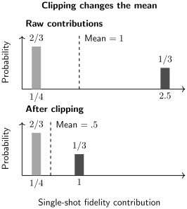
Exact distributions for an ideal Bell state under independent local Pauli choices. The large raw contribution compensates for many unmatched rounds. Clipping it removes that compensation. Bars show probabilities, not a simulated histogram.

The covariance matters even here. The three signed correlator estimators cannot be nonzero on the same shot. Their negative covariances reduce the fidelity variance below the result obtained by treating them as independent (Exercise 3).

If Bell fidelity is the only target, choose one of $XX,YY,ZZ$ uniformly, instead of choosing both local bases independently. Let $t$ be the outcome product, with an extra minus sign for $YY$. Then $(1+3t)/4$ is unbiased for the same $F$ and equals one on every ideal-Bell shot. The better schedule answers a narrower question; it does not determine arbitrary two-qubit coherences.

The measurement map explains the inverse

For a random unitary $U$ followed by computational-basis outcome $b$, define

$$Q_{U,b}=U^\dagger|b\rangle\langle b|U.$$

The ideal ensemble defines the linear map

$$\mathcal M(A)=\mathbb E_U\sum_b \operatorname{Tr}(Q_{U,b}A)\,Q_{U,b}.$$

Averaging the rotated-back projector gives $\mathcal M(\rho)$. If $\mathcal M$ is invertible, define $\widehat\rho=\mathcal M^{-1}(Q_{U,b})$; linearity then proves $\mathbb E\widehat\rho=\rho$.

For uniform one-qubit Pauli measurements,

$$\mathcal M(A)=\frac{A+\operatorname{Tr}(A)I}{3},$$

which yields the factor three above. The inverse is a classical calculation and need not be a physical quantum operation.

For an incomplete ideal design, let $\mathcal S$ be the span of its measured projectors. The map is self-adjoint and positive in the Hilbert–Schmidt inner product, with range $\mathcal S$ and kernel $\mathcal S^\perp$. Its pseudoinverse reconstructs the orthogonal projection of $\rho$ onto $\mathcal S$. Only observables in that visible subspace are determined without further assumptions. An arbitrary chosen subspace is not automatically invariant under the measurement map.

Simultaneous accuracy and median of means

The expectation identity does not by itself bound the error of a finite dataset. For each Hermitian observable, subtract its known identity component:

$$O_0=O-\frac{\operatorname{Tr}O}{d}I.$$

A useful squared shadow norm is the worst-case second moment

$$\|O_0\|_{\mathrm{sh}}^2 =\sup_\sigma\mathbb E_\sigma \left[\operatorname{Tr}(O_0\widehat\rho)^2\right].$$

Suppose this is at most $B$ for each of $M$ specified observables. Then suitable aggregation uses

$$N=O\!\left( \frac{B}{\varepsilon^2} \log\frac{M}{\delta} \right)$$

independent snapshots to estimate all $M$ expectations within additive error $\varepsilon$, with joint failure probability at most $\delta$ (Huang, Kueng, and Preskill, 2020).

One simple construction is median of means. Divide the data into $K$ independent groups of $L$ snapshots. For each observable, calculate its mean within every group, then take the median of those means. Choosing $L\geq4B/\varepsilon^2$ makes each group’s failure probability at most $1/4$ by Chebyshev’s inequality. For odd $K\geq8\log(M/\delta)$, a concentration bound and union bound establish the simultaneous guarantee. Exercise 4 derives these conservative constants.

The median is not generally unbiased, even though each snapshot and group mean is unbiased. Its purpose is a reliable finite-sample error bound.

Targets may be chosen after acquisition without using the observed fluctuations. A guarantee for a fixed finite family also covers selecting a member of that family after looking at the data. Searching an unrestricted new family for the largest fluctuation requires additional analysis or independent held-out data. The cost of evaluating and returning $M$ answers also remains.

Choosing local, biased, or global measurements

For biased independent local basis choices, let $p_i(P)$ be the probability of selecting basis $P$ on qubit $i$. The Pauli-string match probability is

$$q_W=\prod_{i\in S}p_i(W_i).$$

Use the product of outcomes divided by $q_W$ on matching rounds, and zero otherwise. Its second moment is $1/q_W$. Giving important bases more probability can reduce the variance of a known Hamiltonian (Hadfield and colleagues, 2022). Zero coverage makes an incompatible direction unidentifiable.

A deterministic schedule needs an estimator appropriate to its actual match counts. Reusing a randomized inverse with unrelated nominal probabilities is not justified. Derandomized methods construct schedules around a specified target family (Huang, Kueng, and Preskill, 2021).

Global Clifford measurements instead use a uniformly random $n$-qubit Clifford before readout. With $d=2^n$,

$$\widehat\rho=(d+1)Q_{U,b}-I,$$

and the centered-observable bound is

$$\|O_0\|_{\mathrm{sh}}^2 \leq3\operatorname{Tr}(O_0^2).$$

For a rank-one projector, the right-hand side is $3(1-1/d)$, independent of exponential Hilbert-space size. For a nonidentity Pauli string it is $3d$, which is unfavorable compared with local measurements of a short string.

Design	Useful when	Main limitation
Local Pauli	Many low-weight correlators matter	Match cost grows with weight
Targeted product bases	A known list dominates the task	Other directions may be absent
Global Clifford	Low-rank global observables matter	Entangling circuits and query cost

A global snapshot can be stored as a stabilizer tableau, but an overlap with an arbitrary target state need not be efficiently computable. Compact storage and low copy complexity do not guarantee efficient classical queries.

Local marginals, nonlinear properties, and noise

Estimating all Pauli strings of weight at most $k$ determines every $k$-qubit reduced operator. A convenient upper bound on the number of coordinates is $M\leq\binom nk4^k$. For fixed $k$, the simultaneous coordinate-wise copy bound grows logarithmically with $n$.

Coordinate error is not trace-distance error. If every nonidentity coefficient of a $k$-qubit marginal has error at most $\varepsilon$, Pauli orthogonality and a matrix-norm inequality give

$$\frac12\|\widehat\rho_A-\rho_A\|_1 \leq\frac12\sqrt{4^k-1}\,\varepsilon.$$

This is a bound on the reconstructed Hermitian operator, which need not be positive. A subsequent physical projection is another estimator and needs its own analysis. Exercise 6 derives the bound.

Pure-target fidelity is linear in $\rho$; purity is not. For independent snapshots, an unbiased purity estimate is

$$\widehat{\mathcal P} =\frac1{N(N-1)} \sum_{r\neq s}\operatorname{Tr} (\widehat\rho^{(r)}\widehat\rho^{(s)}).$$

Using distinct snapshots avoids self-pairing bias. The linear-observable theorem does not automatically give the variance of this estimator, nor guarantees for entropy, negativity, or mixed-state fidelity.

Noise changes what must be inverted. Let $\widetilde{\mathcal M}(\rho)$ denote the mean of the recorded nominal projectors under the actual noisy experiment. Applying the ideal inverse yields

$$\mathbb E\widehat\rho_{\mathrm{ideal}} =\mathcal M^{-1}\widetilde{\mathcal M}(\rho).$$

Calibration can correct an invertible noisy map under a specified noise model, but weak response directions amplify variance and calibration uncertainty. Robust-shadow protocols make these assumptions explicit (Chen and colleagues, 2021). Exercise 7 gives an exact readout example.

If the preparation drifts, randomized bases must remain independent of the current prepared state for a per-shot inverse to target that state in expectation. Correlated data need a different confidence analysis. Outcome-dependent rejection can also change the accepted ensemble differently for different bases. Keep basis choices, outcomes, and times so these effects can be tested.

Shadow tomography in its original sense

Aaronson’s original shadow-tomography problem asks for the probabilities of many known two-outcome measurements on an unknown state. His 2018 revised bound has polylogarithmic dependence on the number of targets and Hilbert-space dimension, but uses a different, demanding quantum-measurement model with collective operations.

Classical shadows instead use randomized measurements on individual copies and pay an observable-dependent variance cost. The two results should not be treated as the same algorithm. Full state tomography remains necessary when the goal is a uniformly accurate description of arbitrary state directions.

Exercises

1. A missing measurement direction

Only $X$ and $Z$ are measured, each with probability one half. Determine the visible operator subspace and give two indistinguishable qubit states.

Solution

The measured projectors span $\{I,X,Z\}$. The measurement map preserves $I$, scales $X,Z$ by $1/2$, and annihilates $Y$. The states $(I\pm Y)/2$ therefore give identical probabilities. The pseudoinverse recovers their common visible component $I/2$, but cannot recover their opposite $Y$ expectations.

2. Exact Pauli variance and no matches

For a weight-five Pauli query with expectation zero, find the variance of the mean of $N=1000$ uniform local shadows. What is the probability that no round matches its basis?

Solution

The variance is $3^5/1000=0.243$, so the standard deviation is about $0.493$. The match count is binomial with match probability $1/243$, giving

$$\begin{aligned} \Pr(\text{no matches}) &=\left(1-\frac1{243}\right)^{1000}\\ &\approx0.0162. \end{aligned}$$

On such a dataset the usual inverse-probability estimate is zero, even though zero matches do not demonstrate a zero expectation. An error statement must reflect the sampling design.

3. Bell fidelity and covariance

For an ideal Bell state, compute the variance of $\widehat F$. Compare with a calculation that incorrectly treats the three signed correlator estimates as independent.

Solution

Define $A=\widehat x$, $B=-\widehat y$, and $C=\widehat z$. Each has mean one and second moment nine. Different terms cannot be nonzero together, so $\mathbb E(AB)=\mathbb E(AC)=\mathbb E(BC)=0$. Their pairwise covariances are therefore $-1$.

Thus

$$\begin{aligned} \operatorname{Var}(\widehat F) &=\frac{3(9-1)+6(-1)}{16}\\ &=\frac98. \end{aligned}$$

Ignoring covariances would give $24/16=3/2$. Directly using the two-point distribution in the figure gives the same correct variance.

4. Derive a median-of-means guarantee

A single-shot estimator for each of $M$ observables has variance at most $B$. Prove the stated group sizes suffice for joint failure probability at most $\delta$.

Solution

A group mean of $L$ independent shots has variance at most $B/L$. Chebyshev bounds its failure probability by $B/(L\varepsilon^2)\leq1/4$.

For independent groups, the median can fail only if at least half the group means fail. Hoeffding’s inequality applied to their failure indicators gives

$$\Pr(\text{median fails})\leq e^{-K/8}.$$

Choosing odd $K\geq8\log(M/\delta)$ makes this at most $\delta/M$. A union bound over targets gives total failure at most $\delta$. Target estimates may share the same snapshots; independence is needed between groups, not between observables.

5. Biased bases

A two-qubit $ZZ$ target uses independent basis probabilities $p_1(Z)=p_2(Z)=0.8$. Find its second moment and compare with uniform local Pauli shadows. What if a target requires $X$ on a site with $p(X)=0$?

Solution

The match probability is $0.64$, and the matching contribution has magnitude $1/0.64$. Hence the second moment is $1/0.64=1.5625$, compared with nine for uniform sampling. A target with zero match probability is unidentifiable under that design; dividing by zero is not an estimator.

6. From coordinate errors to a matrix bound

Prove the stated trace-norm bound for a reconstructed $k$-qubit marginal whose nonidentity Pauli errors obey $|\Delta r_P|\leq\varepsilon$.

Solution

Let $d_A=2^k$ and $\Delta\rho=d_A^{-1}\sum_{P\neq I}\Delta r_P P$. Orthogonality gives

$$\|\Delta\rho\|_2^2 =\frac1{d_A}\sum_{P\neq I}(\Delta r_P)^2.$$

Using $\|\Delta\rho\|_1\leq\sqrt{d_A}\|\Delta\rho\|_2$ yields

$$\frac12\|\Delta\rho\|_1 \leq\frac12\sqrt{4^k-1}\,\varepsilon.$$

For $k=2$ and $\varepsilon=0.01$, this upper bound is about $0.0194$. It is a sufficient worst-case bound, not a claim that all errors saturate it.

7. Readout correction changes variance

Uniform local Pauli measurements have independent symmetric recorded-sign flips of known probability $q=0.1$ on every measured qubit. For a weight-two target of expectation $\mu$, find the ideal estimator’s mean and the corrected estimator’s variance.

Solution

Two sign flips attenuate the mean by $(1-2q)^2=0.64$. The ideal inverse therefore has mean $0.64\mu$, while its second moment remains nine.

Dividing the contribution by $0.64$ restores mean $\mu$. Its variance becomes

$$\begin{aligned} \operatorname{Var}(\widehat w_{\mathrm{corr}}) &=\frac9{0.64^2}-\mu^2\\ &\approx21.9727-\mu^2. \end{aligned}$$

The noiseless variance was $9-\mu^2$. The second moment is multiplied by $1/0.64^2$, but the variance ratio is not generally that same factor because the mean is restored. Calibration uncertainty is additional.

8. Self-pairing biases purity

For one-qubit Pauli snapshots, show that $\operatorname{Tr}(\widehat\rho^2)=5$. Find the bias of taking the purity of the ordinary snapshot mean.

Solution

The snapshot eigenvalues are $2,-1$, so the trace of the square is $4+1=5$. For $\overline\rho=N^{-1}\sum_r\widehat\rho^{(r)}$, independent distinct pairs have mean overlap $P=\operatorname{Tr}(\rho^2)$. Therefore

$$\mathbb E\operatorname{Tr}(\overline\rho^2) =P+\frac{5-P}{N}.$$

Removing the $N$ self-pairs and dividing by $N(N-1)$ gives the unbiased U-statistic. Its statistical variance still requires analysis.

9. Selecting a query from the data

A simultaneous confidence statement covers a prespecified list of 100 Pauli strings. After inspecting all estimates, a reader reports the largest one. Does this selection invalidate the simultaneous guarantee? What changes if the reader searches additional strings outside the list?

Solution

On the simultaneous-success event every member of the list has a valid error bound, including whichever member was selected. Selection within that covered family preserves the guarantee. Searching outside it is a different statistical problem; the original failure probability does not cover the additional queries. An enlarged-family bound or independent confirmation data is needed.

References

• Aaronson, S. “Shadow tomography of quantum states.” Proceedings of the 50th Annual ACM SIGACT Symposium on Theory of Computing, 325–338 (2018). arXiv:1711.01053.
• Chen, S., W. Yu, P. Zeng, and S. T. Flammia. “Robust shadow estimation.” PRX Quantum 2, 030348 (2021). arXiv:2011.09636.
• Hadfield, C., S. Bravyi, R. Raymond, and A. Mezzacapo. “Measurements of quantum Hamiltonians with locally-biased classical shadows.” Communications in Mathematical Physics 391, 951–967 (2022). arXiv:2006.15788.
• Huang, H.-Y., R. Kueng, and J. Preskill. “Predicting many properties of a quantum system from very few measurements.” Nature Physics 16, 1050–1057 (2020). arXiv:2002.08953.
• Huang, H.-Y., R. Kueng, and J. Preskill. “Efficient estimation of Pauli observables by derandomization.” Physical Review Letters 127, 030503 (2021). arXiv:2103.07510.