Quantum Volume and Application Benchmarks

Quantum volume tests how large a random circuit a quantum computer can execute while retaining a prescribed amount of information about its ideal output. In the usual square-circuit test, a passing width and depth of $m$ gives $V_Q=2^m$. Thus $V_Q=64$ describes a six-qubit, six-layer test, not 64 usable qubits.

The score includes compilation, routing, gates and readout. Application-oriented benchmarks ask a different question: how well does the same system execute circuits drawn from particular workloads? A useful comparison keeps the output quality, elapsed time and resources visible, because one scalar cannot describe all these properties.

Required background. Quantum circuits supplies the gate and measurement model; why benchmarking is hard explains why the measured quantity must match the claim. Helpful background. Probability spaces supplies expectations and conditional probabilities.

Random model circuits and heavy outputs

The model circuit has $m$ qubits, starts in $|0^m\rangle$, and contains $d$ layers. Each layer randomly pairs the qubits and applies an independent Haar-random two-qubit unitary to each pair. One qubit is idle when $m$ is odd. Successive layers use fresh pairings and gates.

These are logical pairings, not assumptions about physical connectivity. A compiler must synthesize the two-qubit operations and route them through the device. Model depth counts these random layers; it need not equal native gate depth or execution time. Cross and colleagues (2019) define this ensemble and its heavy-output test.

For one circuit $U$, calculate its ideal probabilities

$$p_U(x)=|\langle x|U|0^m\rangle|^2.$$

Sort the $D=2^m$ probabilities and take the median, using the average of the two middle values. The heavy outputs are the strings whose ideal probabilities exceed that median:

$$H_U=\{x:p_U(x)>p_{\rm med}(U)\}.$$

The device produces a distribution $q_U$, so its heavy-output probability is

$$h_U=\sum_{x\in H_U}q_U(x).$$

The heavy set is defined from the ideal circuit, not from the measured histogram. The experiment asks how much measured probability lands in that set.

For example, consider

String	Ideal probability	Heavy?
$00$	$0.50$	Yes
$01$	$0.25$	Yes
$10$	$0.15$	No
$11$	$0.10$	No

The median is $(0.15+0.25)/2=0.20$. Ideal sampling gives heavy probability $0.75$. A uniform sampler gives $0.50$, because two of the four strings are heavy. A device producing $(0.40,0.25,0.20,0.15)$ gives $h_U=0.65$.

For a generic distribution without a tie across its middle probabilities, exactly half the strings are heavy. With ties, the strict inequality can select fewer; the uniform baseline is then $|H_U|/D$. In particular, a perfectly uniform ideal distribution has an empty heavy set. Calculate the set rather than forcing half the outcomes into it.

The benchmark tests the ensemble mean

$$h_{m,d}=\mathbb E_U h_U>\frac23.$$

It does not require every random circuit to have $h_U>2/3$. Nor does this probability-mass test certify the entire distribution: a sampler that always returns one known heavy string scores one while ignoring all other outcomes. The prescribed circuit implementation and sampling procedure therefore matter alongside the score.

Why the ideal heavy probability approaches 0.85

For a sufficiently scrambling, large-dimensional circuit, the scaled probability $z=Dp_U(x)$ is approximately exponentially distributed when output labels are chosen uniformly. This is the Porter–Thomas approximation. The median solves

$$1-e^{-z_{\rm med}}=\frac12, \qquad z_{\rm med}=\ln2.$$

An ideal quantum sample favors labels with larger probabilities. Its density of $z$ is therefore $ze^{-z}$, and its heavy probability approaches

$$\begin{aligned} h_{\rm ideal} &\simeq\int_{\ln2}^\infty ze^{-z}\,dz\\ &=\frac{1+\ln2}{2}\simeq0.8466. \end{aligned}$$

Half the labels are heavy, but those labels carry more than half the probability. This explains the interval between the uniform baseline $1/2$, the passing threshold $2/3$, and ideal performance.

Finite circuits need not have this ideal heavy mass. The four-outcome example has $0.75$, for instance. The experiment uses each circuit’s actual median and heavy set, not the asymptotic median $\ln2/D$.

Under the additional distributional model $q=fp+(1-f)u$, with $u$ uniform and half the outputs heavy,

$$h=\frac12+f\left(h_{\rm ideal}-\frac12\right).$$

Using the asymptotic ideal value gives a passing condition $f>1/(3\ln2)\simeq0.4809$. For the four-outcome example, the condition is instead $f>2/3$. This parameter is a mixture weight; heavy-output probability alone does not determine state or process fidelity. Cross-entropy benchmarking develops the related limitations of interpreting a probability score as fidelity.

A statistical pass needs independent circuits

For a fixed shape $(m,d)$, generate $K$ independent circuits and run $S$ shots of each. Let $N_k$ count heavy shots for circuit $k$. Estimate

$$\widehat h_k=\frac{N_k}{S}, \qquad \widehat h=\frac1K\sum_{k=1}^K\widehat h_k.$$

Shots estimate an individual circuit’s heavy probability; new circuits sample variation across the ensemble. If circuits are independent and shots are conditionally independent and stationary,

$$\operatorname{Var}(\widehat h) =\frac{\sigma_h^2}{K}+\frac{v}{KS},$$

where $\sigma_h^2=\operatorname{Var}_U(h_U)$ and $v=\mathbb E_U[h_U(1-h_U)]$. Taking many shots cannot remove the first term.

The original protocol of Cross and colleagues uses $K\geq100$ and the approximate lower value

$$L_{\rm QV} =\widehat h-2\sqrt{\frac{\widehat h(1-\widehat h)}{K}}.$$

A shape passes when $L_{\rm QV}>2/3$. The paper describes this as a nominal 97.5% one-sided, two-sigma rule. It uses a normal approximation, not an exact finite-sample confidence theorem.

Why does $S$ disappear? The rule allows worst-case circuit variation: a circuit could always produce heavy outputs or never produce them. Repeating its shots would then supply no new independent information. More generally, since a per-circuit fraction lies between zero and one, its variance is at most $h_{m,d}(1-h_{m,d})$; the original rule substitutes the estimated mean into this conservative variance scale.

With $K=100$, $S=1000$ and $\widehat h=0.70$,

$$L_{\rm QV}=0.70-2\sqrt{0.21/100} \simeq0.6083.$$

This does not pass. Incorrectly using $KS=100{,}000$ as the independent sample size would produce approximately $0.6971$ and an unjustified pass.

Other analyses can use observed circuit variation, exact or nonasymptotic intervals, or justified statistical models. State which rule was used; changing it changes the reported statistical test. Resampling complete independent circuit records already includes their measurement fluctuations. Adding a second independent shot-resampling step can count that noise twice. A hierarchical model must instead represent the actual conditional sampling process.

Drift can correlate circuits measured close in time. Randomize their order and repeat across independent time blocks when generalizing across calibrations. Searching many subsets, compiler settings or shapes also requires held-out confirmation or an appropriate selection-aware analysis; a per-shape interval alone does not protect every selected result.

Quantum volume and the width–depth map

Let $d_\star(m)$ be the greatest depth through which the required tests at width $m$ pass. The original width–depth summary is

$$\log_2V_Q=\max_m\min\{m,d_\star(m)\}.$$

The common square-test implementation measures $m=d$ and reports $2^{m^\star}$ for the largest passing square size $m^\star$. Keep the tested shapes and pass margins alongside the score. A pass at an unmeasured shape cannot be inferred merely by drawing a smooth frontier through other measurements.

For two illustrative systems, suppose the passing depths are

Width	System A	System B
$2$	$12$	$6$
$3$	$8$	$5$
$4$	$5$	$4$
$5$	$3$	$3$
$6$	$2$	$2$

Both have largest passing square size four and $V_Q=16$. Yet A supports twice B’s depth at width two. The scalar loses this distinction.

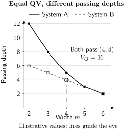
Equal quantum volume does not mean equal performance at every circuit shape. The points use the illustrative table; connecting lines guide the eye. The marked square-test point $(4,4)$ passes for both systems. Neither system passes the next tested square, $(5,5)$.

Volumetric benchmarking, developed by Blume-Kohout and Young (2020), retains independent width and depth and specifies the circuit family and success criterion at every shape. It can reveal narrow/deep and wide/shallow strengths, including nonmonotonic behavior caused by placement or compilation.

The familiar picture of a filled square underneath a frontier assumes a downward-closed capability region. Do not fill holes in an irregular measured map by assumption. A conservative contiguous frontier and the raw pass/fail cells answer different questions; show which is being summarized.

Depth also depends on representation. A random two-qubit model layer, a layer in a standardized comparison gate set, and a layer in a device’s native schedule are different quantities. A map for random circuits does not automatically predict Fourier transforms, simulation, mid-circuit measurement, or error-correction cycles at the same nominal shape.

Compilation and classical reference calculations

Quantum volume intentionally measures the delivered system. The compiler may search placements, optimize synthesis, use native interactions and trade approximation error against additional noisy gates. Improving those choices can legitimately improve the score. Cross and colleagues require the implementation to approximate the requested unitary, rather than replace it with an unrelated circuit chosen to emit heavy strings.

Consequently, a larger score need not mean intrinsically better physical gates. A comparison of complete systems may permit each its best compiler; a more hardware-focused comparison must control compilation choices as far as the architectures allow. In either case, the approximation tolerance, search budget and chosen qubits affect the interpretation.

The reference calculation is another resource. Exact state-vector simulation stores $2^m$ amplitudes, and determining the exact median generally requires information about all ideal output probabilities. Tensor-network methods can change practical costs for favorable circuits, but do not remove the dependence on circuit structure. A classically verified quantum-volume result is a system benchmark, not a demonstration that its circuits are classically intractable.

Application circuits need a task-specific score

An application-oriented suite substitutes named algorithms or subroutines for generic random circuits and sweeps their sizes. Lubinski and colleagues (2023) give one such suite. A circuit inspired by an application may be useful for diagnosis even when its instances are easy to solve classically.

The score should reflect the output the user needs: an energy error, an optimization value, a success probability, or a distributional distance. The same input instances and quality target are needed for meaningful timing comparisons. For example, a 1 ms execution with energy error 0.02 does not meet a 0.01 target; a 3 ms execution with error 0.005 does. The faster run has not solved that specified task.

Two timing measurements may also answer different questions. Scheduled QPU time isolates device execution; elapsed time to an accepted answer can include compilation, communication, classical optimization and verification. Compare matching boundaries and include rejected or failed attempts. Algorithmic benchmarking develops complete task execution and retry costs; resource estimation distinguishes quantum and classical resources.

One suite score deserves particular care. Lubinski and colleagues use the squared classical fidelity

$$F_s(p,q)=\left(\sum_x\sqrt{p_xq_x}\right)^2.$$

For uniform $u$, define $b=F_s(p,u)$ and normalize it as

$$\begin{aligned} F_{\rm raw}&=\frac{F_s(p,q)-b}{1-b},\\ F&=\max\{F_{\rm raw},0\}. \end{aligned}$$

This convention makes ideal sampling score one and uniform sampling score zero when $p$ is nonuniform. It is a distribution score, not a state or process fidelity. It is also nonlinear in $q$, so it is not generally the ideal fraction in a mixture.

If $p=u$, then $b=1$ and the denominator vanishes. Near uniformity, the small denominator amplifies estimation errors. Clipping hides how far below the baseline a result lies: for $p=(0.9,0.1)$ and $q=(0,1)$, $b=0.8$ and $F_{\rm raw}=-3.5$, whereas the clipped score is zero. Retain the raw value when interpreting failures. Finite-shot histogram estimates of this nonlinear statistic can themselves be biased.

Finally, distributional similarity need not equal task success. If a task accepts either $00$ or $11$, always producing $00$ succeeds every time but does not reproduce a uniform distribution over the two accepted answers. Choose the metric to match the question. Report per-task behavior before averaging a suite, since a high mean can hide an entire failed task class.

Exercises

1. Calculate the heavy set

For the four-outcome table, find the median, ideal heavy probability, and heavy probability for $q=(0.40,0.25,0.20,0.15)$. Would always returning $00$ establish faithful sampling?

Solution

The middle values are $0.15$ and $0.25$, so the median is $0.20$. The heavy set is $\{00,01\}$, giving ideal mass $0.75$ and measured mass $0.65$. Always returning $00$ scores one but has total-variation distance $1-p(00)=0.5$ from the ideal distribution. Heavy mass alone does not establish faithful sampling.

2. Ties at the median

Take $p=(0.4,0.2,0.2,0.2)$. What are its heavy set and uniform baseline? Why would arbitrarily choosing the two largest entries change the test?

Solution

The median is $0.2$. Only the first entry is strictly larger, so the uniform baseline is $1/4$ and the ideal heavy mass is $0.4$. Selecting an additional tied entry replaces the stated strict-median rule with a different acceptance set. Neither the $1/2$ baseline nor the Porter–Thomas ideal mass applies to this distribution.

3. Exact and asymptotic mixture thresholds

Under $q=fp+(1-f)u$, find the threshold on $f$ for the four-outcome table and for the Porter–Thomas approximation.

Solution

The table gives $h=0.75f+0.5(1-f)=0.5+0.25f$. Thus $h>2/3$ requires $f>2/3$. In the asymptotic model,

$$\begin{aligned} h&=\frac12+\frac{f\ln2}{2},\\ f&>\frac1{3\ln2}\simeq0.4809. \end{aligned}$$

The different thresholds reflect different ideal distributions. Neither calculation infers quantum process fidelity without additional assumptions.

4. More shots or more circuits?

Let circuit heavy probabilities be $0.6$ or $0.8$ with equal probability. For $K=100$ and $S=1000$, calculate the standard error of the ensemble mean and compare it with a pooled independent-shot calculation.

Solution

The mean is $0.7$, the between-circuit variance is $0.01$, and $v=(0.24+0.16)/2=0.20$. Therefore

$$\begin{aligned} \operatorname{Var}(\widehat h) &=\frac{0.01}{100}+\frac{0.20}{100000}\\ &=0.000102. \end{aligned}$$

The standard error is about $0.01010$. Pooling as independent Bernoulli shots gives $\sqrt{0.21/100000}\simeq0.001449$, almost seven times smaller. Additional circuits reduce both variance terms; additional shots reduce only the second.

5. Apply the original passing rule

Suppose $\widehat h=0.75$ from $K=200$ independent circuits with equal shot counts. Does the original two-sigma rule pass?

Solution

There are at least 100 circuits, and

$$\begin{aligned} L_{\rm QV} &=0.75-2\sqrt{0.75(0.25)/200}\\ &\simeq0.6888>2/3. \end{aligned}$$

It passes this approximate rule. This conclusion assumes the stated independent sampling and does not address an uncorrected search over many candidate results.

6. The same scalar, different capabilities

Compute the two quantum volumes from the width–depth table. Can either system’s score alone predict the quality of a width-two, depth-ten application circuit?

Solution

For A the values of $\min(m,d_\star(m))$ are $2,3,4,3,2$; B has the same values. Both give $V_Q=16$. A passes the random-model shape $(2,10)$ in the illustrative table while B does not. Even that information does not determine performance on a different application circuit family.

7. A normalized score is not a mixture weight

Take $p=(1,0)$, $u=(1/2,1/2)$ and $q=fp+(1-f)u$. Find the normalized classical fidelity. Then explain why the equality with $f$ is not general.

Solution

Here $F_s(p,q)=q_0=(1+f)/2$ and $b=1/2$, giving $F_{\rm raw}=f$. This works because the target is deterministic. For a nondeterministic target the square-root cross terms remain. For example, $p=(0.9,0.1)$ and $f=1/2$ give $q=(0.7,0.3)$ and

$$\begin{aligned} F_s&=(\sqrt{0.63}+\sqrt{0.03})^2\\ &\simeq0.93495,\\ F_{\rm raw}&\simeq0.67477. \end{aligned}$$

This differs from the mixture weight $0.5$.

8. Task success versus distribution fidelity

A task accepts either $00$ or $11$. Let the reference distribution be $p=(1/2,0,0,1/2)$ and the device always output $00$. Find task success, $F_s$, and the normalized score using the four-outcome uniform baseline.

Solution

Task success is one. The distribution fidelity is $F_s=1/2$, and the uniform baseline is also $b=1/2$, so $F_{\rm raw}=0$. The device reliably produces an accepted answer but does not sample the requested reference distribution. These are distinct tasks; the correct score depends on which one was intended.

9. An aggregate can reverse a ranking

Two systems have scores $A=(0.9,0.4)$ and $B=(0.6,0.8)$ on two tasks. For a weighted mean giving weight $w$ to the first task, when is A preferred?

Solution

The means are $0.4+0.5w$ and $0.8-0.2w$. Thus A is preferred when $0.7w>0.4$, or $w>4/7$. Equal weights favor B, whereas sufficiently emphasizing the first task favors A. A suite ranking encodes a choice of workload weights.

References

• Blume-Kohout, R., and K. C. Young. “A volumetric framework for quantum computer benchmarks.” Quantum 4, 362 (2020). doi:10.22331/q-2020-11-15-362.
• Cross, A. W., L. S. Bishop, S. Sheldon, P. D. Nation, and J. M. Gambetta. “Validating quantum computers using randomized model circuits.” Physical Review A 100, 032328 (2019). arXiv:1811.12926.
• Lubinski, T., and colleagues. “Application-oriented performance benchmarks for quantum computing.” IEEE Transactions on Quantum Engineering 4, 3100316 (2023). arXiv:2110.03137.