Process Tomography

Quantum process tomography estimates how a device transforms input states. Preparing a spanning set of known states and measuring their outputs determines a linear map; fitting all counts together can enforce the constraints of a physical quantum channel. Unlike state tomography, both the input preparations and the output measurements must be characterized.

The discussion assumes a finite-dimensional, repeatable operation. A deterministic channel is completely positive and trace preserving (CPTP). A heralded branch instead needs a trace-nonincreasing map, and an operation with memory may require more than one input–output channel.

Required background. State tomography supplies measurement design and statistical estimation; the Choi matrix supplies complete-positivity and trace constraints. Quantum channels explains the equivalent matrix representations.

Four input states determine a qubit map

For each known preparation $\rho_k$, measure several output observables. The probabilities are

$$p(a|k,s)= \operatorname{Tr}\!\left[E_{a|s}\mathcal E(\rho_k)\right],$$

where $E_{a|s}$ is a calibrated measurement effect. For a qubit, a useful input family consists of the projectors onto

$$|0\rangle,\quad |1\rangle,\quad |+\rangle,\quad |+i\rangle.$$

Here $|+\rangle=(|0\rangle+|1\rangle)/\sqrt2$ and $|+i\rangle=(|0\rangle+i|1\rangle)/\sqrt2$. Denote their four output density matrices by $\sigma_0,\sigma_1,\sigma_+,\sigma_{+i}$. Linearity gives

$$\begin{aligned} \mathcal E(I)&=\sigma_0+\sigma_1,\\ \mathcal E(Z)&=\sigma_0-\sigma_1,\\ \mathcal E(X)&=2\sigma_+-\sigma_0-\sigma_1,\\ \mathcal E(Y)&=2\sigma_{+i}-\sigma_0-\sigma_1. \end{aligned}$$

Every qubit operator is a linear combination of $I,X,Y,Z$, so these measurements determine the map. This is the basic prepare-and-measure construction of Chuang and Nielsen (1997).

The output states must be measured, not assumed to remain pure. Independent fits of the four outputs may produce valid density matrices whose linear extension is not completely positive. If all four fitted outputs have trace one, however, that spanning extension is already trace preserving. Complete positivity is the additional, joint consistency condition (Exercise 3).

If an imperfect gate under investigation also prepares the nominal $|+\rangle$ probe, that preparation cannot simultaneously be treated as an independently known reference.

The Choi matrix makes joint reconstruction linear

Use the unnormalized, output–input convention:

$$\begin{aligned} |\Omega\rangle&=\sum_i|i\rangle|i\rangle,\\ J_{\mathcal E} &=(\mathcal E\otimes\operatorname{id}) (|\Omega\rangle\langle\Omega|). \end{aligned}$$

The first factor is the output; the second is a reference copy of the input. Then

$$\begin{aligned} \mathcal E(\rho) &=\operatorname{Tr}_{\mathrm{in}} \!\left[J_{\mathcal E}(I\otimes\rho^{\mathsf T})\right],\\ p(a|k,s) &=\operatorname{Tr}(J_{\mathcal E}M_{a|k,s}),\\ M_{a|k,s}&=E_{a|s}\otimes\rho_k^{\mathsf T}. \end{aligned}$$

The transpose uses the input basis defining $|\Omega\rangle$. It matters for complex probes: for the identity channel, omitting it changes the predicted probability of projecting $|+i\rangle$ onto itself from one to zero.

A deterministic physical channel satisfies

$$J\succeq0,\qquad \operatorname{Tr}_{\mathrm{out}}J=I_{\mathrm{in}}.$$

In particular, $\operatorname{Tr}J=d_{\mathrm{in}}$. The normalized Choi state is $J/d_{\mathrm{in}}$, whose input-reference marginal is $I_{\mathrm{in}}/d_{\mathrm{in}}$.

For dimensions $d_{\mathrm{in}}$ and $d_{\mathrm{out}}$, the CPTP set has interior dimension

$$d_{\mathrm{in}}^2(d_{\mathrm{out}}^2-1).$$

A Hermitian Choi matrix starts with $d_{\mathrm{in}}^2d_{\mathrm{out}}^2$ real parameters; the partial-trace equation imposes $d_{\mathrm{in}}^2$ independent real constraints. Positivity limits their range but does not lower the interior dimension.

The preparation and measurement design must distinguish all trace-preserving perturbations $\Delta J$ satisfying $\operatorname{Tr}_{\mathrm{out}}\Delta J=0$. Spanning input states and informationally complete output measurements suffice. Very small singular values in this linear design still make inversion unstable.

A bit-flip example and a coherent alternative

Consider the one-parameter channel

$$\mathcal E_q(\rho)=(1-q)\rho+qX\rho X.$$

The flip probability satisfies $0\leq q\leq1$.

Its Bloch-vector action is

$$\begin{aligned} r_x'&=r_x,\\ r_y'&=(1-2q)r_y,\\ r_z'&=(1-2q)r_z. \end{aligned}$$

Thus the four ideal probe outputs have Bloch vectors

Input	Output Bloch vector
$\lvert0\rangle$	$(0,0,1-2q)$
$\lvert1\rangle$	$(0,0,-1+2q)$
$\lvert+\rangle$	$(1,0,0)$
$\lvert+i\rangle$	$(0,1-2q,0)$

If $920$ of $1000$ measurements on the $|0\rangle$ output give outcome zero, the bit-flip model gives $\widehat q=0.08$. Its approximate binomial standard error is $\sqrt{0.08(0.92)/1000}\approx0.00858$.

That one experiment does not establish the bit-flip model. A coherent rotation

$$U_\theta=e^{-i\theta X/2}, \qquad \cos\theta=1-2q=0.84,$$

gives the same $Z$ probabilities on input $|0\rangle$. For $0<\theta<\pi$, however,

$$\begin{aligned} \langle Y\rangle_{\text{bit flip}}&=0,\\ \langle Y\rangle_{\text{rotation}} &=-\sin\theta\approx-0.543. \end{aligned}$$

The stochastic output has a shorter Bloch vector; the unitary output remains pure.

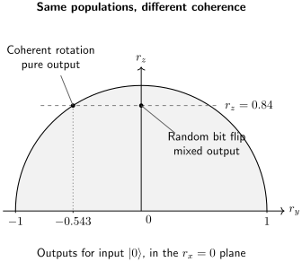
Both channels return the same $Z$ contrast, $0.84$, on input $|0\rangle$. Measuring $Y$ separates their outputs. One population measurement cannot determine the off-diagonal information needed for a channel estimate.

For the bit-flip model, write $|A\rangle\!\rangle=(A\otimes I)|\Omega\rangle$. Its Choi matrix is

$$J_q={}(1-q)|I\rangle\!\rangle\langle\!\langle I| +q|X\rangle\!\rangle\langle\!\langle X|.$$

The normalized matrix $J_q/2$ has eigenvalues $1-q,q,0,0$. Relative to the identity, $F_e=1-q$ and

$$F_{\mathrm{avg}}=\frac{2F_e+1}{3} =1-\frac{2q}{3}\approx0.9467.$$

The coherent alternative has the same average fidelity, despite its different action. Fidelity is a scalar summary, not a reconstruction of the error.

Estimation, constraints, and uncertainty

With fixed input–setting counts and independent stationary trials, use the multinomial log-likelihood

$$\ell(J)=\sum_{k,s,a}n_{a|k,s} \log\operatorname{Tr}(JM_{a|k,s}).$$

Maximizing this concave function over $J\succeq0$ with the correct partial trace gives a physical maximum-likelihood estimate (Fiurášek and Hradil, 2001). Zero-count terms contribute zero. A positive count assigned zero probability makes $\ell=-\infty$.

Linear inversion is useful for exposing poorly determined directions, but can give negative Choi eigenvalues. Constrained least squares and projected least squares use different objectives; projection depends on its norm and weighting. Surawy-Stepney and colleagues (2022) study specific projected estimators and their statistical guarantees.

Low-rank or near-unitary assumptions can reduce the number of unknowns, but must be tested against additional data. A commonly suggested shortcut does not work: for positive trace-preserving Choi matrices,

$$\|J\|_*=\operatorname{Tr}J=d_{\mathrm{in}}.$$

The nuclear norm is constant on the feasible set, so adding a multiple of it to a CPTP fitting objective cannot favor low Kraus rank. Useful rank restrictions require a genuinely different model or objective.

Uncertainty must describe the quantity being reported. For a $d$-dimensional CPTP map and target unitary $U$, the output–input Choi convention gives

$$F_e=\frac{\operatorname{Tr}(J_{\mathcal E}J_U)}{d^2}, \qquad F_{\mathrm{avg}}=\frac{dF_e+1}{d+1}.$$

Here $F_e$ uses the squared-fidelity convention with the pure normalized target Choi state; the average-fidelity relation is general for CPTP maps, not restricted to bit flips (Nielsen, 2002). In the one-parameter example, the approximate standard error of $F_{\mathrm{avg}}$ is $(2/3)\operatorname{se}(\widehat q)\approx0.00572$, conditional on the bit-flip and calibration assumptions.

A full channel confidence region permits bounds on these linear fidelities by optimization over the region. A point estimate of diamond distance is not itself a guaranteed experimental upper bound. Refer to hardware metrics for the meanings of these quantities.

Ancilla assistance changes the experiment

Prepare a known maximally entangled state of the input and a reference:

$$|\Phi\rangle=\frac1{\sqrt d}\sum_i|i\rangle_S|i\rangle_R.$$

Applying the process only to $S$ produces $J_{\mathcal E}/d$. Joint state tomography therefore reconstructs the channel from one type of joint input. Many repeated preparations and joint measurement settings are still needed.

More generally, expand the known input state in an operator-Schmidt decomposition,

$$\sigma_{SR}=\sum_{\ell=1}^{R}s_\ell A_\ell\otimes B_\ell.$$

One input is faithful for unrestricted process reconstruction when the input-side operators span all $d_{\mathrm{in}}^2$ directions, equivalently $R=d_{\mathrm{in}}^2$ with nonzero coefficients. Small coefficients amplify uncertainty when inverted. Entanglement is not necessary: certain separable correlated states are faithful (Altepeter and colleagues, 2003; Exercise 5). Conversely, an entangled pure state supported on only two levels of a three-level input misses the remaining directions.

For an $n$-qubit channel, the generic CPTP dimension is $16^n-4^n$. Conventional product probes with local Pauli readout use $4^n3^n=12^n$ preparation–setting configurations. Ancilla assistance with local Pauli readout uses $3^{2n}=9^n$ settings on $2n$ qubits. These are design counts, not shot counts, and the enlarged state preparation and measurement can be demanding.

Randomized benchmarking answers a narrower question about sequence decay. Choi-state shadow methods can estimate selected process properties. Neither provides an arbitrary channel at uniformly accurate precision with polynomial resources in $n$.

Preparation errors, memory, and successful branches

If all nominal inputs experience the same preparation map $\mathcal P$, and all output effects share an imperfection representable by a map $\mathcal M$ before ideal readout, the data identify

$$\mathcal E_{\mathrm{eff}} =\mathcal M\circ\mathcal E\circ\mathcal P.$$

They do not separate the three factors. Preparation-dependent or setting-dependent errors need not even admit this single composite-map description. More shots improve precision within the assumed model; they do not identify missing calibration information.

Gate-set tomography fits preparations, measurements, and gates together from sequences. In Liouville coordinates, an invertible change

$$\begin{aligned} |\rho\rangle\!\rangle&\mapsto G|\rho\rangle\!\rangle,\\ \langle\!\langle E|&\mapsto\langle\!\langle E|G^{-1},\\ \mathcal G_i&\mapsto G\mathcal G_iG^{-1} \end{aligned}$$

leaves sequence probabilities unchanged. This algebraic gauge freedom means individual coordinates are not directly observed; not every arbitrary transformation preserves a chosen physical parameterization. Nielsen and colleagues (2021) explain gauge choices and statistical analysis. See also SPAM errors.

A channel fitted to one use does not automatically predict repeated uses. Suppose a hidden bit chooses either $I$ or $Z$ with equal probability and remains fixed for two uses. Every one-use experiment sees dephasing, but two uses apply either $I^2$ or $Z^2$, both identity. Squaring the fitted dephasing channel would predict dephasing again. Repeated-sequence tests detect this memory; non-Markovian noise explains the more general setting.

For a successful branch $\mathcal K$, retain unnormalized outputs and success counts. Its Choi matrix obeys

$$J_{\mathcal K}\succeq0,\qquad \operatorname{Tr}_{\mathrm{out}}J_{\mathcal K}\preceq I.$$

The normalized conditional output is

$$\rho_{\mathrm{succ}} =\frac{\mathcal K(\rho)}{\operatorname{Tr}\mathcal K(\rho)}.$$

When success depends on the input, this expression is generally nonlinear in $\rho$ and must not be fitted as an ordinary channel. It becomes linear after division by a common success probability only when that probability is state independent.

Additional probe states, repeated settings, and sequences test these assumptions. Compare measured and predicted probabilities by preparation, time, and context. A constrained fit always produces a physical matrix; agreement on observations outside the fit determines whether that matrix is useful for prediction.

Exercises

1. Count channel parameters

Find the CPTP interior dimension for a qubit channel and a channel from a qubit to a three-level system.

Solution

A Hermitian Choi matrix has $d_{\mathrm{in}}^2d_{\mathrm{out}}^2$ coordinates. Its fixed input marginal imposes $d_{\mathrm{in}}^2$ real constraints. Thus the two dimensions are $4(4-1)=12$ and $4(9-1)=32$. Full-rank positive Choi matrices exist in both cases, so positivity does not reduce these interior dimensions.

2. Test the transpose with a complex probe

For the identity channel, calculate the probability of projecting input $|+i\rangle$ onto $|+i\rangle$ using the Choi formula. What happens without the input transpose?

Solution

For $J_{\mathrm{id}}=|\Omega\rangle\langle\Omega|$,

$$\langle\Omega|A\otimes B|\Omega\rangle =\operatorname{Tr}(AB^{\mathsf T}).$$

With $E=\rho=|+i\rangle\langle+i|$, the correct choice $B=\rho^{\mathsf T}$ gives $\operatorname{Tr}(\rho^2)=1$. Omitting the transpose gives $\operatorname{Tr}(\rho\rho^{\mathsf T})=0$, since $\rho^{\mathsf T}=|-i\rangle\langle-i|$. Real probes alone would miss this mistake.

3. Four physical outputs need not define a channel

Suppose the four probe outputs are the transposes of their inputs. Are they physical? Is the spanning linear extension CPTP?

Solution

Each transposed density matrix is positive and trace one. The extension is the transpose map, which fixes $I,X,Z$ and sends $Y$ to $-Y$. It preserves trace, but its Choi matrix is the swap operator. Swap has eigenvalue $-1$ on the antisymmetric Bell state, so the extension is not completely positive. Checking each output separately misses this joint requirement.

4. Equal populations, different coherence

For $q=0.08$, find the positive $Y$-measurement probability on input $|0\rangle$ after the bit-flip channel and after $U_\theta$ with $\cos\theta=0.84$.

Solution

The bit-flip output has $\langle Y\rangle=0$, so $p_Y(+)=1/2$. The rotated output has

$$\begin{aligned} \langle Y\rangle&=-\sqrt{1-0.84^2},\\ p_Y(+)&=\frac{1-\sqrt{1-0.84^2}}2\\ &\approx0.2287. \end{aligned}$$

Both have $p_Z(0)=0.92$. Measuring the complementary basis detects their coherence difference.

5. A faithful separable probe

Let $|s\rangle$ range over the six Pauli eigenstates and let $|s^*\rangle$ denote computational-basis conjugation. Show that

$$\sigma=\frac16\sum_s |s\rangle\langle s|\otimes|s^*\rangle\langle s^*|$$

is separable and faithful for qubit process tomography.

Solution

It is explicitly a mixture of product states, hence separable. Pairing the positive and negative eigenstates of each axis gives

$$\sigma={}\frac{I\otimes I}{4} +\frac{X\otimes X-Y\otimes Y+Z\otimes Z}{12}.$$

The four independent input operators $I,X,Y,Z$ all have nonzero coefficients. Thus the operator-Schmidt rank is four. Process inversion is possible, although the three traceless correlations are smaller than for a maximally entangled probe, which increases noise amplification.

6. Why nuclear-norm regularization fails here

Compare the nuclear norms of the unnormalized Choi matrices for the identity channel and complete depolarization $\rho\mapsto I/d$. Can that norm distinguish their Kraus ranks under CPTP constraints?

Solution

The identity Choi matrix is $|\Omega\rangle\langle\Omega|$, with one eigenvalue $d$. The depolarizing Choi matrix is $I_{d^2}/d$, with $d^2$ eigenvalues $1/d$. Both have nuclear norm $d$, despite ranks one and $d^2$. Every positive trace-preserving Choi matrix has the same norm, so the penalty is constant.

7. Separate a gate error from a preparation error?

A nominal input is followed either by a bit flip of probability $0.1$ during preparation and a perfect device, or by perfect preparation and a device bit flip of probability $0.1$. Can arbitrary output measurements distinguish the two cases?

Solution

Both produce exactly the same output for every nominal input. Standard process tomography identifies the same composite channel in both cases. More choices of output measurement or more shots cannot separate the factors without additional preparation information.

8. A normalized successful branch is nonlinear

Take $K=\operatorname{diag}(1,1/2)$ and $\mathcal K(\rho)=K\rho K^\dagger$. Compare conditioning after applying $\mathcal K$ to $I/2$ with the equally weighted mixture of the conditioned $|0\rangle$ and $|1\rangle$ outputs.

Solution

The success probabilities are $1$ and $1/4$ for $|0\rangle$ and $|1\rangle$. Their individually normalized outputs remain those pure states, whose equal mixture is $I/2$.

For the mixture sent through the operation, however,

$$\mathcal K(I/2)= \operatorname{diag}(1/2,1/8).$$

Success probability is $5/8$, giving conditioned output $\operatorname{diag}(4/5,1/5)$. Conditioning reweights the ensemble toward the more successful input. The linear object is $\mathcal K$, including its trace.

9. Detect memory with two uses

For the persistent hidden $I/Z$ choice described above, compare the probability of measuring $X=+1$ on input $|+\rangle$ after two actual uses and after applying the fitted one-use channel twice.

Solution

The actual two-use operation is identity for either hidden choice, giving probability one. The one-use fitted map is $\mathcal D(\rho)=(\rho+Z\rho Z)/2$. It sends $|+\rangle\langle+|$ to $I/2$ and obeys $\mathcal D^2=\mathcal D$, giving probability $1/2$. One-use data cannot distinguish persistent from freshly resampled noise.

10. Five-qubit resource counts

Calculate the generic CPTP dimension, conventional product preparation–setting count, and ancilla-assisted local Pauli setting count for five qubits.

Solution

The counts are

$$\begin{aligned} 16^5-4^5&=1{,}047{,}552,\\ 12^5&=248{,}832,\\ 9^5&=59{,}049. \end{aligned}$$

The last experiment measures a ten-qubit output state, so fewer distinct configurations do not by themselves establish a lower laboratory cost. Repeated shots, calibration, and joint preparation are additional resources.

References

• Altepeter, J. B., D. Branning, E. Jeffrey, T. C. Wei, P. G. Kwiat, R. T. Thew, J. L. O’Brien, M. A. Nielsen, and A. G. White. “Ancilla-assisted quantum process tomography.” Physical Review Letters 90, 193601 (2003). doi:10.1103/PhysRevLett.90.193601.
• Chuang, I. L., and M. A. Nielsen. “Prescription for experimental determination of the dynamics of a quantum black box.” Journal of Modern Optics 44, 2455–2467 (1997). doi:10.1080/09500349708231894.
• Fiurášek, J., and Z. Hradil. “Maximum-likelihood estimation of quantum processes.” Physical Review A 63, 020101(R) (2001). doi:10.1103/PhysRevA.63.020101.
• Nielsen, E., J. K. Gamble, K. Rudinger, T. Scholten, K. Young, and R. Blume-Kohout. “Gate set tomography.” Quantum 5, 557 (2021). doi:10.22331/q-2021-10-05-557.
• Nielsen, M. A. “A simple formula for the average gate fidelity of a quantum dynamical operation.” Physics Letters A 303, 249–252 (2002). doi:10.1016/S0375-9601(02)01272-0.
• Surawy-Stepney, T., J. Kahn, R. Kueng, and M. Guţă. “Projected least-squares quantum process tomography.” Quantum 6, 844 (2022). doi:10.22331/q-2022-10-20-844.