Verification of Quantum Advantage

A quantum-advantage experiment compares a quantum method with classical methods on the same computational task. Two questions must be answered together: did the device produce the requested result, and what did that result cost compared with the classical alternatives? A hardness theorem can explain why the task is promising, but its assumptions must match the experiment. This page develops those distinctions through small examples; it does not rank present-day devices.

Required background. Algorithmic benchmarking explains accepted answers, retries and complete runtime. Quantum complexity classes distinguishes complexity assumptions from algorithm timings.

Helpful background. Cross-entropy benchmarking explains one sampling statistic; circuit simulation introduces classical alternatives.

Correct answers and computational advantage

Suppose a quantum device returns two factors of a large integer. Multiplication checks the answer cheaply. That success establishes correctness, but an advantage comparison still needs a classical factoring method and comparable resources. Conversely, a fast device returning incorrect factors has not solved the task.

The same separation appears in less easily checked problems:

Requested output	Useful check	What remains uncertain
Factors or another witness	Evaluate the defining relation	Cost of finding it classically
An optimized configuration	Check feasibility and objective value	Distance from the optimum
An expectation value	Compare with a reliable reference or bound	Reference error and estimator bias
Samples from a distribution	Test specified distributional properties	Properties the tests do not constrain
An interactive response	Apply a protocol with a soundness theorem	Whether its assumptions hold

A query advantage compares calls to a specified oracle. A finite runtime advantage compares implementations at selected problem sizes. A practical advantage additionally concerns a useful complete task. Oracle construction, state preparation, error correction and verification can change the relationship between these statements. The benchmarking review by Proctor and colleagues explains why a device score needs an explicit computational interpretation.

An empirical comparison can be convincing without a proven lower bound against every classical algorithm. It should then say which classical methods were evaluated. A mathematical separation makes the stronger claim only within the model and assumptions of its theorem.

Why sampling is harder to check

For a target distribution $p$ and observed distribution $q$, total-variation distance is

$$\operatorname{TV}(p,q)=\frac12\sum_z|p(z)-q(z)|.$$

It equals the largest difference between their probabilities of any event. Thus small total variation controls every event, whereas agreement on a few averages controls only those averages.

Consider two-bit outcomes in the order $00,01,10,11$:

$$\begin{aligned} p&=(1/4,1/4,1/4,1/4),\\ q&=(1/2,0,0,1/2). \end{aligned}$$

Each individual bit is equally likely to be zero or one under either distribution. A verifier measuring only single-bit frequencies sees perfect agreement. Nevertheless, $\operatorname{TV}(p,q)=1/2$: equal bits occur with probability $1/2$ under $p$ and probability one under $q$.

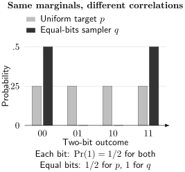
Matching both single-bit distributions leaves a large difference in their joint distribution. The parity test distinguishes these examples immediately. For $n$ bits, the uniform distribution and the uniform distribution on even-parity strings agree on every marginal involving fewer than $n$ bits, yet remain a total-variation distance $1/2$ apart.

More diagnostics can detect more failure modes, but a finite list needs a mathematical connection to the desired conclusion. Secret tests can reduce deliberate tuning; secrecy alone does not supply that connection. A classical program that cheaply passes the actual test is relevant to a claim about passing that test, even if its mechanism differs from the device.

A sample-complexity limitation

In ordinary identity testing, the target $p$ is fully known and one receives independent samples from an otherwise unrestricted $q$. At fixed success probability, the worst-case number of samples needed to distinguish $q=p$ from $\operatorname{TV}(p,q)\geq\epsilon$ scales as

$$N=\Theta\!\left(\frac{\sqrt D}{\epsilon^2}\right)$$

for $D$ possible outputs. This is a promise-testing result, not a universal confidence interval for an arbitrary nearby $q$. Valiant and Valiant give the stronger, target-dependent theory: concentrated targets can be much easier. Testing a point mass, for example, needs only $O(1/\epsilon)$ samples at constant confidence, independently of $D$.

For a broad $n$-bit target, $D=2^n$ makes even the square-root scaling exponential in $n$. Evaluating the target probabilities can add another computational difficulty. Additional trusted measurements, structural assumptions or interaction can change the verification problem; a lower bound for ordinary samples does not rule those methods out.

What a hardness argument actually says

An exact amplitude can be hard to calculate even when a noisy experiment is easy to imitate. Approximate sampling therefore needs its own argument. A common route combines hardness of approximating output probabilities on typical instances, an approximate-counting reduction, and assumptions about classical complexity classes. Anticoncentration ensures that a substantial fraction of probabilities are not too small relative to $1/D$; it helps translate certain additive errors into relative ones. It is neither sufficient for hardness nor a universal prerequisite for every sampling-hardness proof. These distinctions are developed by Hangleiter and Eisert.

The uniform distribution illustrates the point: all probabilities equal $1/D$, so it anticoncentrates perfectly, yet independent fair bits sample it efficiently. Likewise, one difficult instance does not establish difficulty for a randomly drawn population. A worst-case theorem, an average-case conjecture and a measured runtime are different kinds of statements.

Noise changes the requested approximation

For a simple illustrative mixture, let $u$ be uniform and

$$q_f=fp+(1-f)u,\qquad 0\leq f\leq1.$$

Direct substitution gives

$$\begin{aligned} \operatorname{TV}(q_f,u)&=f\operatorname{TV}(p,u),\\ \operatorname{TV}(q_f,p)&=(1-f)\operatorname{TV}(p,u). \end{aligned}$$

If $\operatorname{TV}(p,u)=0.4$ and $f=0.02$, uniform samples approximate the physical output within $0.008$, while the physical output remains $0.392$ from the ideal target. Whether that device passes depends on which distribution and tolerance the task specifies. Small nonzero correlation with $p$ is compatible with both facts.

This mixture is a model, not a general description of circuit noise. In general, the noisy output cannot even be inferred from the ideal output probabilities alone: those probabilities discard phases and intermediate states. Noise simulation works with channels and circuits that retain the necessary information. Noise can simplify some tasks, but no general rule says every noisy quantum computation is easy.

Comparing classical and quantum costs

At a fixed accuracy, confidence and instance population, let $C_a$ be the cost of classical method $a$. For the evaluated set $\mathcal A$, define

$$C_{\mathrm{tested}}=\min_{a\in\mathcal A}C_a.$$

If $C_{\mathrm{opt}}$ is the optimum over all allowed classical algorithms, then

$$C_{\mathrm{opt}}\leq C_{\mathrm{tested}}.$$

The measured cost supplies an upper bound on the best possible classical cost. Taking its ratio to a quantum time does not reverse that inequality. A timeout on one method likewise gives no lower bound on another method’s cost. For a randomized method, one timed-out run is merely a censored observation of its completion time; it does not even establish that method’s mean runtime.

The comparison should include useful domain-specific approximations and methods aimed at the actual acceptance rule. Asking a classical program to compute the full state while asking the quantum device only for a few observables compares different outputs. Tensor-network simulation explains why geometry and requested observables can matter more than the full Hilbert-space dimension.

A quality mismatch can reverse the ranking

Suppose, purely as a calibrated example, two unbiased independent-sampling estimators have root-mean-square errors

$$\begin{aligned} \sigma_Q(T)&=\sqrt{0.05/T},\\ \sigma_C(T)&=\sqrt{0.002/T}. \end{aligned}$$

Here $T$ is in seconds and setup cost is negligible. The quantum estimator reaches $0.10$ in $5$ s; the classical estimator reaches $0.01$ in $20$ s. Comparing just those times suggests a fourfold quantum improvement. At the common error $0.10$, however, the classical time is $0.2$ s, which is 25 times faster. Equal error and confidence must precede the time comparison. The example assumes the displayed scaling is valid; biased or correlated estimators need a different analysis.

Preprocessing, retries, discarded shots and verification belong in the chosen timing boundary. Reusable setup can be amortized across a batch when both methods receive that opportunity. Energy and financial comparisons require their own measured boundaries; a short circuit does not determine whole-system energy use.

If improved classical software changes its cost from $1000$ s to $20$ s while a quantum task takes $10$ s, the ratio changes from $100$ to $2$. The original timings remain historical facts. The updated comparison answers a different, later question.

Statistical uncertainty and the tested population

For paired instances with positive costs, define

$$\ell_i=\log(C_{C,i}/C_{Q,i}),\qquad \Delta=\mathbb E[\ell_i].$$

Then $e^\Delta$ is a geometric-mean cost ratio. It is not the ratio of mean costs and does not imply a win on every instance. At large enough sample size, with an appropriate standard error, an approximate one-sided lower bound is

$$L=\exp[\widehat\Delta-z_{1-\alpha}\operatorname{SE}(\widehat\Delta)].$$

For paired data, covariance matters. Write $L_C=\log C_C$ and $L_Q=\log C_Q$:

$$\begin{aligned} \operatorname{Var}(\overline L_C-\overline L_Q)&=v_C+v_Q-2c,\\ c&=\operatorname{Cov}(\overline L_C,\overline L_Q). \end{aligned}$$

Here $v_C,v_Q$ are variances of the two sample means. Heavy tails, timeouts and changing hardware can invalidate the simple approximation. Repeated shots from one circuit do not supply new independent circuit instances; uncertainty must reflect the population to which the conclusion applies.

Choosing the best result among many settings also changes the inference. For $K$ prespecified tests, assigning each a false-positive allowance $\alpha/K$ controls the chance of any false positive by the union bound, without requiring independence. Inspecting results repeatedly until a fixed-sample interval becomes favorable needs a valid sequential method instead. A statistical confidence level concerns the tested comparison; it cannot assign a probability that no undiscovered classical algorithm exists.

Verification through interaction

Interaction lets a verifier ask challenges that a static output file cannot answer. A test of quantumness separates an honest quantum device from a specified class of classical strategies. A verification protocol for computation bounds acceptance of an incorrect computational result, including attacks by a dishonest quantum prover. These are different soundness requirements.

Brakerski and colleagues construct tests and randomness protocols from suitable cryptographic functions. Mahadev gives classical verification of quantum computations under a learning-with-errors hardness assumption against efficient quantum algorithms. The precise adversary and security assumptions matter; a result about classical attackers should not be silently promoted to security against quantum attackers.

For illustration, suppose a protocol bounds the conditional success probability of every allowed classical strategy by $s$ on every round, including conditioning on its previous history. Independent fresh challenges plus that conditional bound permit concentration arguments even if the device has memory. For scores $X_j\in\{0,1\}$,

$$\Pr\!\left[\frac1N\sum_jX_j\geq s+\eta\right] \leq e^{-2N\eta^2}.$$

One cannot insert a single-round bound into this formula without establishing its applicability after earlier rounds. Cryptographic composition may also contribute a security error. Verifier time, communication, rejected rounds and physical overhead still matter to a resource advantage.

For conventional hardware tests, combine independently checked small instances, physically informative observables and fresh data at the target scale. Agreement in an easy regime supports a model but does not prove its extrapolation across an unexplained transition. Verification of quantum simulation develops complementary physical checks; reproducible notebooks explains how another reader can rerun a calculation.

Exercises

1. A marginal test misses parity

For the two-bit distributions in the figure, calculate both single-bit probabilities, the equal-bits probability and total variation. Extend the conclusion to uniform even-parity strings on $n$ bits.

Solution

Both single-bit probabilities of one are $1/2$. Equal bits have probabilities $1/2$ and $1$, and the four absolute differences are each $1/4$, giving total variation $1/2$. Fixing any $k<n$ bits leaves $2^{n-k-1}$ even-parity completions, so every such marginal has probability $2^{-k}$. The full parity still differs.

2. A concentrated target

The target always outputs $0$. A wrong sampler outputs something else with probability at least $\epsilon=0.1$. How many independent samples make the probability of missing all discrepancies at most $0.05$?

Solution

The worst miss probability is $(1-\epsilon)^N$. Therefore

$$N\geq\frac{\log0.05}{\log0.9}\approx28.43.$$

Use $N=29$. For small $\epsilon$, this is approximately $\log(20)/\epsilon$, regardless of the number of possible wrong strings. This does not contradict a worst-case bound over targets.

3. A noisy target

For the mixture above, suppose $\operatorname{TV}(p,u)=0.4$. At what $f$ does uniform sampling meet a $0.01$ tolerance around $q_f$? At what $f$ does $q_f$ meet that tolerance around $p$?

Solution

The first condition is $0.4f\leq0.01$, hence $f\leq0.025$. The second is $0.4(1-f)\leq0.01$, hence $f\geq0.975$. Approximating the noisy device and implementing the ideal task are very different requirements here.

4. A timeout and a new algorithm

A classical program times out at $1000$ s; the quantum method takes $10$ s. Another classical method completes the same task in $5$ s. What can be concluded?

Solution

That run of the first program exceeded $1000$ s. The second method proves the optimal classical cost is at most $5$ s, so the quantum method is not faster than the evaluated classical alternatives. Neither the timeout nor the size of the state vector proves a universal classical lower bound.

5. Paired uncertainty

Let $\widehat\Delta=\log5$, standard errors of the two mean log costs be $0.12,0.08$, and their correlation be $0.75$. Find the approximate 95% one-sided lower ratio using $z=1.645$.

Solution

The covariance is $0.75(0.12)(0.08)=0.0072$. Thus

$$\begin{aligned} v_\Delta&=0.0144+0.0064-0.0144,\\ \operatorname{SE}(\widehat\Delta)&=\sqrt{v_\Delta}=0.08,\\ L&=5e^{-1.645(0.08)}\approx4.38. \end{aligned}$$

Setting covariance to zero would give about $3.94$. Pairing removes shared instance difficulty in this example; it does not remove uncertainty about untested algorithms.

6. Geometric means and total time

Two equally likely instances have classical times $(100,1)$ s and quantum times $(10,5)$ s. Compute the geometric-mean speedup and ratio of mean times.

Solution

The ratios are $10$ and $0.2$, with geometric mean $\sqrt2\approx1.414$. The ratio of means is $50.5/7.5\approx6.733$. The quantum method loses on the second instance. The two averages answer different questions.

7. Conditional success against memory

A hypothetical test has conditional classical success bound $s=0.75$. In $N=1000$ rounds, the observed fraction is $0.85$. Evaluate the stated concentration bound. Why is a marginal single-round bound insufficient?

Solution

The bound is $e^{-20}\approx2.06\times10^{-9}$. If all outcomes instead equal one shared Bernoulli variable with success probability $0.75$, each round has marginal success $0.75$, but all rounds succeed with probability $0.75$. After an early success, the conditional bound fails. A valid protocol must exclude that failure of the premise.

8. Fixed mitigation weights

For $Y=2A-B$, let $\operatorname{Var}(A)=\operatorname{Var}(B)=0.01$ and $\operatorname{Cov}(A,B)=0.006$. Calculate the variance. What changes if the weights are fitted to these same data?

Solution

For fixed weights and finite second moments,

$$\begin{aligned} \operatorname{Var}(Y)&=4(0.01)+0.01-4(0.006)\\ &=0.026. \end{aligned}$$

This covariance identity is exact; independence would instead give $0.05$. Data-dependent weights are random and can correlate with $A,B$, so simply substituting fitted weights omits their uncertainty and possible bias. Probabilistic error cancellation discusses sampling costs for signed estimators.

9. Extrapolating a control

A device reproduces all Clifford control circuits, but has an untested coherent error on a non-Clifford gate. Does control agreement establish correctness of circuits using that gate? Does anticoncentration establish classical hardness?

Solution

Neither conclusion follows. The controls did not exercise the faulty operation; target validation needs sensitivity to it or a justified bound on its error. Uniform independent bits provide an efficiently sampled, perfectly anticoncentrated distribution. Additional computational structure and a relevant hardness argument are needed.

References

• Brakerski, Z., Christiano, P., Mahadev, U., Vazirani, U., and Vidick, T. “A cryptographic test of quantumness and certifiable randomness from a single quantum device.” Journal of the ACM 68, article 31 (2021). doi:10.1145/3441309; arXiv:1804.00640.
• Hangleiter, D., and Eisert, J. “Computational advantage of quantum random sampling.” Reviews of Modern Physics 95, 035001 (2023). doi:10.1103/RevModPhys.95.035001.
• Mahadev, U. “Classical verification of quantum computations.” In 59th IEEE Symposium on Foundations of Computer Science, pp. 259–267 (2018). doi:10.1109/FOCS.2018.00033; arXiv:1804.01082.
• Proctor, T., Young, K., Baczewski, A. D., and Blume-Kohout, R. “Benchmarking quantum computers.” Nature Reviews Physics 7, 105–118 (2025). doi:10.1038/s42254-024-00796-z.
• Valiant, G., and Valiant, P. “An automatic inequality prover and instance optimal identity testing.” SIAM Journal on Computing 46, 429–455 (2017). doi:10.1137/151002526.