Reporting Standards

A quantum result becomes useful when a reader can tell what was measured, which conditions it describes, and how precisely it is known. “Fidelity 99.7%” or “runtime 90 seconds” leaves those questions open. This guide shows how to describe a result well enough to interpret, compare and recompute it, using small numerical examples.

Helpful background. Why benchmarking is hard explains the role of task and population; device characterization explains how fitted parameters depend on a physical model. Reproducible notebooks develops the practical computation checks.

A measured quantity needs a precise question

Begin with the physical object and the quantity being estimated. For a gate, name the target operation and distinguish average gate fidelity from a fitted randomized-benchmarking decay parameter. For an energy, specify the Hamiltonian, units and reference energy. For a logical error rate, distinguish failure per experimental shot from a rate inferred per correction round. Hardware metrics explains these definitions.

Then describe the population: which qubits, circuits, input instances, calibration period and experimental conditions the result averages over. A good compact statement might read:

For this fixed circuit and qubit pair, 6,840 of 10,000 attempted trials produced an accepted correct output. The acceptance rule was fixed before acquisition. Of the 7,200 accepted trials, 95.0% were correct; 68.4% of all attempts were accepted and correct.

The two percentages answer different questions. A report should also say how correctness was checked, when the trials were collected and whether their independence is plausible. With independent, identically distributed trials, an approximate standard error for the all-attempt success fraction is

$$\begin{aligned} \operatorname{SE}(\widehat p) &\approx\sqrt{\frac{0.684(1-0.684)}{10000}}\\ &\approx0.00465. \end{aligned}$$

An approximate 95% normal interval is therefore $0.684\pm0.0091$. It describes sampling uncertainty under that model; it does not cover a biased correctness detector or changes on a different day. Near zero or one, use an appropriate binomial interval instead of this normal approximation. The NIST handbook gives several constructions.

The population can reverse a comparison

Suppose two systems attempt different mixtures of easy and hard instances. The entries below are successful attempts divided by total attempts.

Instance class	System A	System B
Easy	90/100 = 90%	19/20 = 95%
Hard	2/10 = 20%	24/80 = 30%
All recorded attempts	92/110 ≈ 83.6%	43/100 = 43%

B has a higher observed success fraction in each class, yet A has a higher pooled fraction because A mostly tried easy instances. The pooled results are valid summaries of their respective datasets; they do not compare the same task distribution.

For a target distribution with equal weight on the two classes, use

$$\begin{aligned} \widehat p_A&=(0.90+0.20)/2=0.55,\\ \widehat p_B&=(0.95+0.30)/2=0.625. \end{aligned}$$

These are descriptive estimates, not a demonstration that their difference is statistically resolved. In particular, A has only ten hard-instance attempts. State the intended weights before comparing systems and propagate uncertainty within each class.

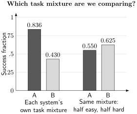
Changing the question changes the average. The left pair uses each system’s own mixture of tasks. The right pair applies the same 50:50 mixture to both. Bars show the calculated point estimates above; they omit uncertainty to isolate the effect of weighting.

The same issue arises when one experiment selects its best qubit pair, another averages all pairs, or two algorithms use different input distributions. Keep per-instance results so readers can compare an appropriate shared population.

Uncertainty follows the experiment

Circuits and shots are different random units

Suppose $K$ circuits are sampled independently from an ensemble, and each receives $n$ independent shots. Let $P_k$ be circuit $k$‘s true success probability and $Z_k$ its measured fraction. The law of total variance gives

$$\begin{aligned} \operatorname{Var}(Z_k) &=\operatorname{Var}(P_k) +\frac{\mathbb E[P_k(1-P_k)]}{n},\\ \operatorname{Var}(\overline Z) &=\frac{\operatorname{Var}(Z_k)}{K}. \end{aligned}$$

The sample variance of the observed $Z_k$, divided by $K$, estimates this total variance for identically distributed circuit records. It already includes shot noise. Adding a separate shot-noise estimate to it counts that contribution again. A hierarchical model can instead estimate the components separately and combine them once.

Taking more shots reduces the second term but cannot replace sampling more circuits. If the circuits are a fixed list and only repeated-shot uncertainty is wanted, condition on that list: the between-circuit population term then answers a different question. Shared calibration drift can also correlate circuits, invalidating the independent-circuit formula. Report acquisition order and independent time blocks when that matters.

Statistical spread and model limitations

Label every error bar: standard deviation across instances, standard error of a mean, a confidence interval with stated coverage, or a Bayesian interval with its prior. A frequentist 95% confidence procedure covers the fixed parameter in 95% of repeated experiments under its assumptions; it does not assign a posterior probability to the parameter after observing one interval.

For calibrated inputs $\boldsymbol\theta$ and a differentiable reported quantity $q=f(\boldsymbol\theta)$, first-order propagation uses the full covariance matrix $\Sigma$:

$$u_q^2\approx(\nabla f)^{\mathsf T}\Sigma\nabla f.$$

The JCGM guide explains this treatment of correlated inputs. Near a singularity or boundary, linear propagation can fail; numerical propagation must still use a justified input distribution and measurement model.

An unknown model bias is not automatically an independent Gaussian error bar. If a separate argument guarantees an additive bias of magnitude at most $b$, enlarge a valid statistical interval $[L,U]$ to $[L-b,U+b]$. If $b$ is itself uncertain, its guarantee needs to be included. Numerical convergence alone does not bound omitted physical effects.

Selection and data processing change the result

State the acceptance rule and retain counts for rejected as well as accepted attempts. Setting-dependent or outcome-dependent selection may change the population. A high accepted-state fidelity should therefore appear beside its acceptance fraction. For Bell tests, selection also affects the validity of the classical bound; see entanglement certification.

When many layouts, optimizers or seeds are tried, show their distribution and selection cost. The best noisy score tends to look better than its underlying performance. Use fresh measurements of the selected configuration for a final estimate, and distinguish that estimate from expected performance over a new optimization run.

Error mitigation changes the estimator. Give raw and transformed results, coefficients or fit choices, calibration inputs, covariance and total shots. A linear combination

$$\widehat q=\sum_j a_j\widehat q_j$$

has variance $\mathbf a^{\mathsf T}\Sigma\mathbf a$. Clipping a result to a physical interval changes its bias and sampling distribution. It must be stated and included when assessing uncertainty; an unphysical uncorrected estimate can be informative about statistical variation or model failure.

Time and resources need the same boundary

Name the timed operation: circuit execution, a complete job, or an accepted answer including compilation, optimization, retries and verification. Give classical and quantum costs where both contribute. Measured costs and projected fault-tolerant costs should be visibly distinguished.

For repeated independent attempts with constant success probability $p>0$ and mean attempt cost $\overline C$, the mean cost to first success is

$$\mathbb E[C_{\mathrm{total}}]=\overline C/p.$$

Success and cost may be correlated within an attempt: the formula still holds when the cost–success pairs are identically distributed and independent across attempts. This follows by conditioning on the first attempt, then restarting the same process after failure. Correlated failures, changing policies or a finite retry limit need a different calculation. Algorithmic benchmarking gives the fuller time-to-solution analysis.

For energies, an error relative to exact diagonalization of a chosen active-space Hamiltonian measures accuracy for that model. It does not include basis truncation, the active-space approximation or neglected relativistic effects. Chemistry case studies illustrates why both the problem definition and its computational cost matter.

Make the result possible to recompute

Preserve the data needed for the stated analysis, the analysis and plotting code, and exact software versions with instructions for running them. Include the executed circuit or enough compilation settings to reconstruct it; source circuits alone may omit routing and scheduling changes. A random seed needs its generator and version. Keep numerical plot data, units, setting labels and trial order when order affects the inference. Sandve and colleagues explain these practical reproducibility habits.

Following the National Academies’ terminology, reproducibility checks computations with the same inputs and methods, while replicability compares results from newly collected data. Reproducing a figure does not independently confirm the device model. Describe which check was actually performed.

Cite a fixed data and code release. If a correction changes an estimate, preserve the earlier version and explain the change in a new release. A file digest can help identify the bytes used, but cannot establish their scientific correctness.

Some data cannot be public. Explain what is unavailable, how eligible readers can request access, and which conclusions cannot be independently checked without it. The FAIR principles permit authenticated access; they also call for useful metadata and reuse conditions. Restricted data should not prevent release of unrestricted counts, circuits and analysis code.

Exercises

1. Change the target distribution

Using the comparison table, let the target probability of an easy instance be $w$. Can A outperform B at any common $0\leq w\leq1$ according to these point estimates?

Solution

$$\begin{aligned} \widehat p_A(w)&=0.20+0.70w,\\ \widehat p_B(w)&=0.30+0.65w,\\ \widehat p_B(w)-\widehat p_A(w)&=0.10-0.05w>0. \end{aligned}$$

B has the larger point estimate for every common mixture. A’s larger pooled score used a different mixture. Sampling uncertainty still matters when inferring true performance.

2. Count circuit and shot uncertainty once

Half the circuits have true success probability $0.2$ and half $0.8$. Sample $K=50$ circuits independently and take $n=100$ shots per circuit. Find the variance of their mean measured fraction.

Solution

The circuit probabilities have mean $0.5$ and variance $0.09$. In either class $P(1-P)=0.16$, so

$$\operatorname{Var}(\overline Z) =\frac{0.09+0.16/100}{50}=0.001832.$$

The standard error is about $0.0428$. Treating all 5,000 shots as independent Bernoulli draws with probability $0.5$ would give only $0.00707$. The shots are conditionally independent within a circuit, but share its random success probability.

3. Zero failures is not zero risk

No failures occur in $N=1000$ independent trials with fixed failure probability $p$. Derive the exact one-sided 95% binomial upper confidence limit for this observation.

Solution

Solve $(1-p_{\mathrm U})^{1000}=0.05$:

$$p_{\mathrm U}=1-0.05^{1/1000}\approx0.002991.$$

Probabilities above this value make the observed zero failures a less than 5% event. The result is the zero-count endpoint of a binomial confidence procedure, not a claim of perfect reliability.

4. Select the best noisy energy

Two candidates have the same true energy $E$. Each estimate independently equals $E-\delta$ or $E+\delta$ with equal probability. What is the mean of the smaller reported estimate? What changes with an independent final measurement of the selected candidate?

Solution

The minimum is $E+\delta$ only when both estimates are high, an event of probability $1/4$. Otherwise it is $E-\delta$. Its mean is $E-\delta/2$. A fresh unbiased measurement has mean $E$ because its noise is independent of selection. It does not erase the cost of trying both candidates or quantify variation in a new optimization campaign.

5. Include costs of failed attempts

An attempt succeeds with probability $0.25$. Success takes 8 seconds and failure 2 seconds. Attempts are independent. Find the expected time to first success.

Solution

There are on average three failures before the success, giving $3(2)+8=14$ seconds. Equivalently,

$$\overline C=0.25(8)+0.75(2)=3.5\ \mathrm{s},$$

and $\overline C/0.25=14$ seconds. Using the successful-run duration divided by success probability would incorrectly give 32 seconds.

6. Expand an interval for bounded bias

A statistical 95% interval for a measured quantity is $[0.70,0.74]$. Independent of the observed data, a valid physical bound limits the additive calibration bias to $0.01$ in magnitude. Give an interval for the bias-free quantity with at least the same coverage.

Solution

Use $[0.69,0.75]$. Whenever the statistical interval covers the biased mean, this expanded interval covers every allowed bias-free value. Adding $0.01$ in quadrature would require a probabilistic interpretation that the bound alone does not provide.

7. Preserve paired measurements

Across three independent test instances, A’s scores are $(0.4,0.6,0.8)$ and B’s are $(0.5,0.7,0.9)$. Compare the observed standard error of the mean paired difference with one obtained by treating the systems’ scores as independent.

Solution

Every paired difference is $0.1$, so its sample standard error is zero. Each system separately has sample variance $0.04$; ignoring the pairing gives

$$\begin{aligned} \operatorname{SE}_{\mathrm{unpaired}} &=\sqrt{(0.04+0.04)/3}\\ &\approx0.1633. \end{aligned}$$

The covariance cancels the shared variation in difficulty. Three identical observed differences do not establish zero population variance, and shot uncertainty may still remain. The point is to preserve the actual pairing and describe what the error bar includes.

8. Distinguish an even number of logical flips

A logical bit flips independently with probability $r$ in each of $R$ rounds. Only its final value is measured. Derive the final failure probability and explain why dividing it by $R$ is generally incorrect.

Solution

The final value is wrong after an odd number $F$ of flips. Since $\mathbb E[(-1)^F]=(1-2r)^R$,

$$p_{\mathrm{final}}=\frac{1-(1-2r)^R}{2}.$$

For $r=0.1$ and $R=10$, this is about $0.4463$, not $Rr=1$. The approximation $p_{\mathrm{final}}\approx Rr$ requires $Rr\ll1$ in this model. A measurement of whether any failure occurred would instead have probability $1-(1-r)^R$. State which event the experiment detects.

References

• Joint Committee for Guides in Metrology. Evaluation of Measurement Data—Guide to the Expression of Uncertainty in Measurement. JCGM 100:2008 (2008). doi:10.59161/JCGM100-2008E.
• National Academies of Sciences, Engineering, and Medicine. Reproducibility and Replicability in Science. National Academies Press (2019). doi:10.17226/25303.
• NIST/SEMATECH. e-Handbook of Statistical Methods, §7.2.4.1, “Confidence intervals.” Binomial proportion intervals.
• Sandve, G. K., Nekrutenko, A., Taylor, J., and Hovig, E. “Ten simple rules for reproducible computational research.” PLoS Computational Biology 9, e1003285 (2013). doi:10.1371/journal.pcbi.1003285.
• Wilkinson, M. D., et al. “The FAIR Guiding Principles for scientific data management and stewardship.” Scientific Data 3, 160018 (2016). doi:10.1038/sdata.2016.18.