Interconnects and Transduction

An interconnect transfers quantum information or distributes entanglement between physical nodes. A transducer changes the carrier or frequency used along that path. A cold microwave cable can connect superconducting modules without conversion; a microwave–optical converter can bridge their frequencies to optical fibre. In either case, preserving a coherent classical tone is a weaker test than preserving an unknown qubit or entanglement.

Three quantities must be distinguished: how much signal reaches the output, how much reaches the receiver’s mode, and how much unwanted excitation arrives with it. This page develops these hardware questions. Quantum Teleportation and Quantum Repeaters explain the protocols that use such links.

Required background. Hardware Overview introduces device operations; Bits, Qubits, Qudits, and Modes distinguishes encodings; Quantum Channels and Noise provides the channel description of a lossy transfer.

Coherent transfer and heralded entanglement

For direct transfer, the receiver starts in a known state. In a single-rail encoding, an ideal operation has the action

$$(\alpha|0\rangle_A+\beta|1\rangle_A)|0\rangle_B \longmapsto |0\rangle_A(\alpha|0\rangle_B+e^{i\phi}\beta|1\rangle_B).$$

The phase $\phi$ must be stable and corrected or tracked. Emission, conversion, propagation, and capture together determine this map; efficient conversion inside one resonator does not establish efficient transfer between nodes. Cirac and colleagues give a cavity-based construction, while Kurpiers and colleagues demonstrate shaped microwave emission and capture.

Loss in the vacuum/one-photon encoding produces amplitude damping: an absent photon is indistinguishable from the logical $|0\rangle$. In a dual-rail one-photon encoding, the two-mode vacuum lies outside the code and can in principle identify loss. A practical nondestructive flag requires an appropriate detector, ancillary system, or subsequent protocol; destructive photon detection cannot leave the same unknown flying qubit available for use.

In heralded entanglement, photons correlated with two local memories interfere at a measurement station. A suitable joint outcome announces an entangled memory pair. Cleanly rejected loss lowers the accepted rate; false detections, multiphoton emission, distinguishability, and memory decoherence can also lower the fidelity of accepted pairs. The successful event must not reveal which component of the intended superposition occurred.

The pair can subsequently support teleportation of a data qubit. Its quality can be estimated on separately measured sample pairs; ordinary tomography does not certify each pair while also leaving that same pair intact. Classical notification and memory storage remain necessary. Physical transport of an ion, atom, or electron is another way to connect zones: carrier conversion is absent, but heating, leakage, loss, and path-dependent phase still affect the transported state.

Temporal modes and captured signal

Let $[a_{\rm in}(t),a_{\rm in}^\dagger(t')]=\delta(t-t')$. A normalized envelope defines one bosonic mode,

$$\begin{aligned} A_f&=\int dt\,f^*(t)a_{\rm in}(t), \\ \int dt\,|f(t)|^2&=1. \end{aligned}$$

Then $[A_f,A_f^\dagger]=1$. If the emitted photon has envelope $f$ and the receiver accepts $g$, the captured probability in the absence of other loss is

$$\mu=\int dt\,g^*(t)f(t), \qquad \eta_{\rm mode}=|\mu|^2.$$

The phase of $\mu$ matters for superpositions of vacuum and one photon, and relative phases matter between two encoded rails. Noise or excitations in orthogonal modes cannot automatically be treated as vacuum loss; the vacuum environment assumption must be justified.

For stationary, linear conversion, express frequencies as offsets $\Omega$ from each port’s carrier in its rotating frame. In a number-conserving model,

$$b_{\rm out}(\Omega) =S_{ba}(\Omega)a_{\rm in}(\Omega) +\sum_j S_{bj}(\Omega)v_j(\Omega).$$

The $v_j$ include unused and dissipative input ports. With all such ports included, preservation of the output commutator requires

$$|S_{ba}(\Omega)|^2+\sum_j|S_{bj}(\Omega)|^2=1.$$

Gardiner and Collett develop this input–output description of damped modes.

Here “number conserving” concerns signal excitations after treating the pumps classically. The pumps supply the difference between input and output photon energies. A full active linear transformation can also contain creation operators. A phase-preserving amplifier must introduce idler noise; an ideal single-mode squeezer instead changes the two quadrature noises unequally and need not add an independent environmental mode. See Caves and Continuous-Variable Platforms.

For normalized spectral amplitudes $f(\Omega)$ and $g(\Omega)$, the signal probabilities, with noise counted separately, are

$$\begin{aligned} \eta_{\rm total}&=\int d\Omega\,|S_{ba}(\Omega)f(\Omega)|^2, \\ \eta_{\rm capture}&= \left|\int d\Omega\,g^*(\Omega)S_{ba}(\Omega)f(\Omega)\right|^2 \\ &\le\eta_{\rm total}. \end{aligned}$$

This distinction is useful even for a lossless device. Take a Gaussian spectral intensity of variance $\sigma_\Omega^2$, a quadratic spectral phase $S_{ba}=e^{i\beta\Omega^2/2}$, and a receiver still matched to the original $g=f$. Gaussian integration gives

$$\eta_{\rm total}=1, \qquad \eta_{\rm capture}= \frac{1}{\sqrt{1+\beta^2\sigma_\Omega^4}}.$$

Dispersion has moved part of the signal into modes the receiver rejects. Matching the receiver to the dispersed waveform, or compensating the phase, restores unit capture in this ideal example. Total converted power alone misses the problem.

Pump phase and resonant conversion

With undepleted classical pumps, resonant rotating frames, and a valid rotating-wave approximation, many converters reduce to

$$\frac{H_{\rm conv}}{\hbar} =G a b^\dagger+G^*a^\dagger b.$$

Here $G$ has units of angular frequency. The closed two-mode Heisenberg equations are $\dot a=-iG^*b$ and $\dot b=-iGa$, so, for constant $G=|G|e^{i\varphi}$,

$$\begin{aligned} a(\tau)&=\cos(|G|\tau)a(0) -i e^{-i\varphi}\sin(|G|\tau)b(0),\\ b(\tau)&=\cos(|G|\tau)b(0) -i e^{i\varphi}\sin(|G|\tau)a(0). \end{aligned}$$

At $|G|\tau=\pi/2$, an input $|n\rangle_a|0\rangle_b$ becomes $(-ie^{i\varphi})^n|0\rangle_a|n\rangle_b$. The conversion probability is one, but the number-dependent phase still needs correction for an arbitrary superposition. This is why a pump phase reference is part of coherent state transfer. Lauk and colleagues review the interactions that produce this effective Hamiltonian.

Conversion through an intermediate oscillator

Consider two signal resonators $a,b$ coupled to an intermediate mode $m$ by number-conserving couplings $G_a,G_b$. Let $\kappa_a,\kappa_b$ be total photon-number decay rates and $\gamma_m$ the intermediary’s number decay rate; field amplitudes decay at half these rates. Define

$$C_a=\frac{4|G_a|^2}{\kappa_a\gamma_m}, \qquad C_b=\frac{4|G_b|^2}{\kappa_b\gamma_m}.$$

For steady, resonant, weak signals in the passive linear model, solving the three Langevin equations gives

$$\begin{aligned} \eta_{\rm device} &=\eta_{a,\rm ext}\eta_{b,\rm ext}\eta_{\rm int}, \\ \eta_{\rm int} &=\frac{4C_aC_b}{(1+C_a+C_b)^2}, \\ \eta_{j,\rm ext}&=\frac{\kappa_{j,\rm ext}}{\kappa_j}. \end{aligned}$$

This is a photon-flux efficiency, not an optical-to-microwave power ratio. The derivation assumes Markov damping, no unwanted parametric gain, and signals narrow enough to use the on-resonance value. In a mechanical device, red-detuned drives and resolved sidebands can justify the number-conserving approximation. Off resonance, counter-rotating processes, heating, and finite pulses require the frequency-dependent model rather than this scalar formula.

Eliminating the signal amplitudes at resonance shows the origin of the denominator: the intermediary’s inverse susceptibility is $\gamma_m(1+C_a+C_b)/2$. Both couplings help transfer a signal, but increasing one alone also changes the intermediary’s response. At fixed $C_a$,

$$\begin{aligned} \frac{\partial\eta_{\rm int}}{\partial C_b} &=\frac{4C_a(1+C_a-C_b)}{(1+C_a+C_b)^3}, \\ C_b^{\rm opt}&=1+C_a, \qquad \eta_{\rm int}^{\rm max}=\frac{C_a}{1+C_a}. \end{aligned}$$

Equal, large cooperativities approach unit efficiency. At finite fixed $C_a$, however, exact optimal matching includes the intermediary’s intrinsic loss: $C_b=C_a$ is only an approximation. Pumping the second leg arbitrarily hard eventually reduces conversion. Andrews and colleagues and the Lauk review describe this mechanism.

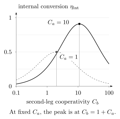
On-resonance internal photon conversion in the passive three-mode model. At fixed $C_a$, increasing $C_b$ helps only up to $C_b=1+C_a$; beyond that point the two conversion legs become mismatched. The horizontal axis is logarithmic. External coupling loss and added thermal photons are not included.

Loss and added photons

The thermal occupation of a mode at angular frequency $\omega$ is

$$\bar n_{\rm th}= \frac{1}{e^{\hbar\omega/(k_{\rm B}T)}-1}.$$

At ordinary laboratory temperatures optical modes have negligible thermal occupation. A well-thermalized $5\ {\rm GHz}$ mode at $20\ {\rm mK}$ is also nearly in vacuum, whereas a $10\ {\rm MHz}$ mechanical mode at the same temperature has $\bar n_{\rm th}\simeq41$. Mechanical damping and cooling must therefore be evaluated at the actual mode frequency. Pump absorption can raise local occupation above the refrigerator thermometer’s value.

For one specified input/output mode pair with signal transmission $\eta>0$, use the normally ordered photon-number convention

$$n_{\rm add}=\frac{n_{\rm out}^{(0)}}{\eta}.$$

Here $n_{\rm out}^{(0)}$ is the physical output occupation with vacuum signal input and the converter operating, including its pumps. Vacuum contributes zero in this convention. A separately calibrated detector background can be removed when inferring the converter’s output; pump-induced photons cannot be subtracted away while claiming a quieter physical channel. Symmetrized quadrature-noise conventions contain vacuum half-quanta and must be converted before comparison. Zeuthen and colleagues formulate the signal/noise distinction for linear transducers.

For a phase-insensitive thermal attenuator,

$$\begin{aligned} b&=\sqrt\eta\,a+\sqrt{1-\eta}\,e, \\ n_{\rm add}&=\frac{(1-\eta)\bar n_e}{\eta}, \end{aligned}$$

where $0<\eta<1$ and $e$ is an independent thermal mode. Holevo’s Gaussian channel criterion gives a precise threshold in this model: it is entanglement breaking exactly when $n_{\rm add}\ge1$. Below that threshold, some input entanglement can survive, but high-fidelity transfer and a positive unassisted quantum capacity do not follow. For example, pure loss has $n_{\rm add}=0$ even at very low transmission. A noise number alone does not establish that an arbitrary, possibly non-Gaussian or phase-sensitive device obeys the thermal-attenuator model.

Pure loss also does not literally replace every input by vacuum with a state-independent probability. A coherent state remains a pure attenuated coherent state. For a single-rail qubit it is amplitude damping, with Kraus operators

$$\begin{aligned} K_0&=|0\rangle\langle0|+\sqrt\eta|1\rangle\langle1|, \\ K_1&=\sqrt{1-\eta}|0\rangle\langle1|. \end{aligned}$$

The average fidelity to ideal transfer over Haar-uniform pure qubits is

$$F_{\rm avg} =\frac{2+\sum_j|\operatorname{Tr}K_j|^2}{6} =\frac{3+2\sqrt\eta+\eta}{6}.$$

This includes all trials and assumes vacuum environment, matched modes, and corrected phase. It is not a conditional detected-photon benchmark. With thermal noise, extra photons can also leave the qubit subspace.

Cascaded stages and reference planes

For independent, phase-insensitive stages satisfying $n_{{\rm out},j}=\eta_j(n_{{\rm in},j}+n_j)$ in compatible modes,

$$n_{\rm add}^{\rm total} =n_1+\frac{n_2}{\eta_1} +\frac{n_3}{\eta_1\eta_2}+\cdots.$$

This follows by substituting each output occupation into the next stage’s input. Earlier loss makes later noise larger when referred back to the original input. Correlated reservoirs, phase-sensitive noise, or frequency mixing require covariance matrices or a full channel model instead.

Likewise, scalar transmissions multiply only for successive matched modes without coherent feedback or multiple-path interference. Two $10\%$ converters and a $50\%$ fibre path then yield $0.5\%$ transmission. Input coupling, filters, and final capture further reduce it. Quoting only internal conversion leaves out these losses. Power transmission differs from photon transmission by $\omega_{\rm out}/\omega_{\rm in}$, with energy supplied or removed by the pump.

Physical conversion mechanisms

Optical frequency conversion

For suitable phase-matched three-wave mixing in a second-order nonlinear medium, a classical pump can produce $\omega_{\rm out}=\omega_{\rm in}\pm\omega_p$. Four-wave Bragg scattering instead exchanges photons between two pumps:

$$\omega_{\rm out}=\omega_{\rm in}+\omega_{p1}-\omega_{p2}.$$

Both processes can yield the number-conserving interaction above. In contrast, degenerate-pump pair generation with $\omega_s+\omega_i=2\omega_p$ produces a signal–idler pair and has a two-mode-squeezing interaction. These are different uses of nonlinear mixing, with different vacuum-noise consequences. Tanzilli and colleagues and McGuinness and colleagues provide examples of state-preserving optical frequency conversion.

Polarization conversion requires matched amplitudes and phases for both polarizations; time-bin conversion requires pump coherence between bins; frequency-bin conversion requires controlled relative spectral phases. Strong pumps can add leakage, Raman photons, and spontaneous pairs. Filtering suppresses some noise but can also reduce capture and distort the waveform. Conversion to telecom wavelengths is helpful only when the resulting fibre advantage outweighs these additional losses and noise for the intended task.

Microwave, mechanical, and atomic interfaces

Mechanism	How the modes couple	Main physical constraint
Direct microwave link	Shaped emission into a cold line and absorption at another circuit	Thermal photons, reflections, and capture shape
Electro-optic conversion	A classical optical pump enhances a Pockels interaction	Weak vacuum coupling, resonance matching, optical heating
Mechanical intermediary	Electrical or piezoelectric coupling and optomechanical coupling share a vibrational mode	Thermal occupation, sideband resolution, and matching the two conversion legs
Atomic or spin-mediated conversion	Driven transitions connect microwave and optical excitations	Population preparation, line broadening, spatial overlap, and fluorescence
Matter–photon interface	State-dependent emission entangles a stationary qubit with light	Collection efficiency and photon indistinguishability

In a direct microwave link, tunable couplers can shape emission for time-reversed absorption. The line and its terminations must remain cold; attenuation at a warm stage injects thermal noise. Cryogenic packaging, isolation, and propagation delay matter even without frequency conversion.

Electro-optic devices avoid a mechanical intermediary. Mechanical devices can provide strong enhanced coupling, but a cold refrigerator is insufficient when the mechanical frequency is low or pump absorption heats the device. Pulsing can reduce average heat at the cost of recovery time and repetition rate. The Han review and Clerk and colleagues develop these alternatives; Mirhosseini and colleagues illustrate coupling a superconducting qubit to a mechanically mediated optical converter.

An ensemble’s collective coupling is $g_{\rm col}=\sqrt{\sum_j|g_j|^2}$ for a properly prepared common ground state and a bright single-excitation mode. It becomes $\sqrt N|g|$ only for equal couplings. This enhancement does not automatically apply to every leg of a multilevel conversion scheme: the populations and the two states connected by that leg matter. Inhomogeneous detunings can transfer the bright excitation into dark collective modes. Cavity QED and Cavity and Circuit QED Frontiers explain the light–matter and hybrid-system mechanisms.

For two independent matter–photon nodes, brightness alone is insufficient. The photons must overlap in spectrum, polarization, and arrival time at the joint measurement. Spectral diffusion, phonon sidebands, and multiphoton emission can degrade the heralded memory state. Photonic Qubits develops interference and detection; Defect and Solid-State Spin Qubits discusses representative emitters.

From a transfer probability to a usable rate

Suppose independent attempts, each with acceptance probability $p$, repeat once per fixed interval $\tau$. The interval includes all preparation, notification, and reset that prevent the next attempt. In this model,

$$R=\frac p\tau, \qquad \mathbb E[T_{\rm first}]=\frac\tau p.$$

These are consequences of a Bernoulli sequence and a geometric waiting time, not general bounds for arbitrary queues, correlated attempts, or pipelined hardware. The propagation time and the classical return path also depend on where the herald is generated. A midpoint station and a far-end receiver have different notification delays; Quantum Memories gives explicit examples.

For $M$ independent usable modes in one round,

$$\begin{aligned} P_{\ge1}&=1-(1-p)^M, \\ \mathbb E[N_{\rm successes}]&=Mp. \end{aligned}$$

The first quantity describes availability of at least one success; the second counts all successes. A receiver that can store only one cannot use the latter as its delivered-pair probability. Mode preparation, switching, detector recovery, memory capacity, and controller timing can all limit multiplexing. See Modular Architectures and Quantum Network Architectures for scheduling and multi-node operation. Kimble gives the broader network setting for these matter–photon interfaces.

Useful measurements therefore pair transfer and noise with a specified mode, input ensemble, phase reference, and trial count. Measure the operating pump noise, not just the pump-off detector floor; include rejected trials in rates and distinguish them from accepted-state fidelity. Check the two directions separately when reflections or pump leakage can disturb the source. These physical tests establish what the link can preserve, beyond showing a coherent output tone.

Exercises

1. Calculate end-to-end transmission

A source emits into a line with probability $0.82$. Input coupling to a converter is $0.70$, internal conversion is $0.55$, output coupling and filtering together are $0.60$, fibre transmission is $0.40$, and target capture is $0.75$. Find the end-to-end transmission.

Solution

The reference-plane factors multiply:

$$\begin{aligned} \eta_{\rm e2e} &= (0.82)(0.70)(0.55) \times (0.60)(0.40)(0.75)\\ &\simeq 0.0568. \end{aligned}$$

Only about $5.7\%$ of source-module trials produce a captured target excitation. Quoting the $55\%$ internal conversion alone would overstate the link transmission by nearly a factor of ten.

2. Refer cascaded noise to the source

Two stages have $\eta_1=0.25$, $\eta_2=0.50$, and input-referred added noises $n_1=0.05$, $n_2=0.10$. What is the total added noise referred to the first input?

Solution

For two stages,

$$\begin{aligned} n_{\rm add}^{\rm tot} &= n_1 + \frac{n_2}{\eta_1} \\ &= 0.05 + \frac{0.10}{0.25} \\ &= 0.45. \end{aligned}$$

The second stage’s noise is magnified by the first stage’s loss. The second stage does not contribute merely $0.10$ when the result is referred to the original source.

3. Compare microwave thermal occupations

Using $h/k_{\rm B}\simeq48.0\ {\rm mK/GHz}$, estimate the thermal occupation of a $5\ {\rm GHz}$ mode at $20\ {\rm mK}$ and at $4\ {\rm K}$.

Solution

The dimensionless ratio is

$$\frac{h\nu}{k_{\rm B}T} = \frac{ (48.0\ {\rm mK/GHz})(5\ {\rm GHz}) }{ T }.$$

At $20\ {\rm mK}$ the ratio is $12$, so

$$\bar n_{\rm th} \simeq \frac{1}{e^{12}-1} \simeq 6.1\times10^{-6}.$$

At $4\ {\rm K}$ the ratio is $0.060$, so

$$\bar n_{\rm th} \simeq \frac{1}{e^{0.060}-1} \simeq 16.2.$$

The same frequency is nearly in its ground state at a well-thermalized $20\ {\rm mK}$ port and highly occupied at $4\ {\rm K}$.

4. Test cooperativity matching

Evaluate the idealized internal efficiency for $(C_a,C_b)=(10,10)$ and $(10,2)$. Then optimize $C_b$ with $C_a=10$ held fixed.

Solution

For equal cooperativities,

$$\eta_{\rm int} = \frac{4(10)(10)}{(1+10+10)^2} = \frac{400}{441} \simeq 0.907.$$

For the mismatched case,

$$\eta_{\rm int} = \frac{4(10)(2)}{(1+10+2)^2} = \frac{80}{169} \simeq 0.473.$$

At fixed $C_a=10$, the derivative changes sign at $C_b=11$, where $\eta_{\rm int}=10/11\simeq0.909$. Equal cooperativities are close to, but not exactly at, this finite-cooperativity optimum. Increasing $C_b$ beyond $11$ decreases conversion in this model.

5. Convert pure loss to average qubit fidelity

An otherwise ideal single-rail transfer has survival probability $\eta=0.36$. Find the average fidelity to the identity for uniformly distributed input qubit states.

Solution

Because $\sqrt{\eta}=0.60$,

$$\begin{aligned} F_{\rm avg} &= \frac{3+2\sqrt{\eta}+\eta}{6} \\ &= \frac{3+1.20+0.36}{6} \\ &= 0.76. \end{aligned}$$

This $76\%$ includes amplitude damping. Selecting only trials in which a photon is detected selects the logical $|1\rangle$ component and destroys an unknown single-rail superposition. It is not a successful heralded transfer of that qubit. Loss flagging must be analyzed with the encoding and the measurement backaction included.

6. Quantify temporal-mode mismatch

The emitted and accepted modes are normalized and have overlap $\mu=0.92e^{i0.3}$. What fraction of the emitted excitation is in the accepted mode? What does the phase mean?

Solution

The mode efficiency is

$$\eta_{\rm mode} = |\mu|^2 = (0.92)^2 \simeq 0.846.$$

About $84.6\%$ lies in the accepted mode. The phase $0.3$ radians is a coherent phase shift of that mode. It can be corrected if stable and calibrated; random drift would instead cause dephasing.

7. Estimate a two-photon heralding rate

Each node produces a usable photon with probability $0.12$ per attempt. Each path and detector together transmit with probability $0.25$. A linear-optical Bell measurement succeeds for half of the two-photon arrivals. Attempts occur at $20\ {\rm kHz}$. Ignore dark events and dead time. Find the heralding rate.

Solution

The probability for one node to deliver a detected photon is

$$p_1 = (0.12)(0.25) = 0.03.$$

The two-photon acceptance probability is

$$p_{\rm acc} = \frac12 p_1^2 = \frac12(0.03)^2 = 4.5\times10^{-4}.$$

Therefore

$$\begin{aligned} R_{\rm acc} &= (2.0\times10^4\ {\rm s}^{-1}) (4.5\times10^{-4}) \\ &= 9\ {\rm s}^{-1}. \end{aligned}$$

The two paths were assumed independent, and the one-half Bell acceptance was specified for this measurement. The quadratic dependence makes modest source or path losses expensive; it is not the scaling of every heralding protocol.

8. Evaluate multiplexed availability

Each of $M=20$ independent frequency bins succeeds with probability $p=0.015$ in one round. Find the probability of at least one success and compare it with the small-$Mp$ approximation.

Solution

The exact probability is

$$\begin{aligned} P_{\ge1} &= 1-(1-0.015)^{20} \\ &= 1-(0.985)^{20} \\ &\simeq 0.261. \end{aligned}$$

The linear approximation gives $Mp=0.30$. It overestimates the exact result because it counts multiple successes in the same round separately. The expected number of successes is exactly $0.30$; it is not the probability of at least one success.

9. Move the noise reference plane

A converter has internal efficiency $0.80$ and internal input-referred noise $0.4$ photons. Add vacuum-loss input coupling $0.05$ and output coupling $0.10$. Find the external signal efficiency and external input-referred noise, assuming independent matched stages.

Solution

The external efficiency is

$$\eta_{\rm ext}=(0.05)(0.80)(0.10)=0.004.$$

For vacuum external input the converter generates $0.80(0.4)=0.32$ photons at its internal output; $0.10(0.32)=0.032$ reach the external output. Thus

$$n_{\rm add}^{\rm ext}=\frac{0.032}{0.004}=8.$$

Output loss attenuates signal and noise equally in this ratio. Input loss attenuates the signal before the internal noise is introduced. Consequently, the internal “less than one added photon” statement does not survive moving the input reference plane. If the full channel is a phase-insensitive thermal attenuator, this external channel is entanglement breaking. Without that model, two scalar measurements alone do not determine its entire action.

10. Recover the pump-dependent swap phase

For $G=|G|e^{i\varphi}$ and $|G|\tau=\pi/2$, find the output of $(\alpha|0\rangle_a+\beta|1\rangle_a)|0\rangle_b$. Give a number-phase rotation that restores the input amplitudes at $b$.

Solution

In the one-excitation basis $(|1,0\rangle,|0,1\rangle)$,

$$H/\hbar=\begin{pmatrix}0&G^*\\G&0\end{pmatrix}.$$

Exponentiating at the swap time gives

$$|0\rangle_a\bigl(\alpha|0\rangle_b-ie^{i\varphi}\beta|1\rangle_b\bigr).$$

Apply $\exp[i(\pi/2-\varphi)n_b]$. The same correction removes the factor $(-ie^{i\varphi})^n$ for every number state, so it also works for a bosonic superposition within the ideal two-mode model. Conversion probability cannot detect a sign error in this phase; a superposition measurement can.

11. Distinguish dispersion from photon loss

A normalized photon has Gaussian spectral intensity with variance $\sigma_\Omega^2$. A converter adds only the phase $e^{i\beta\Omega^2/2}$. For $\beta\sigma_\Omega^2=\sqrt3$, calculate the captured probability in the original mode and the total transmitted probability. How can capture be recovered?

Solution

Writing $x=\Omega/\sigma_\Omega$ and $c=\beta\sigma_\Omega^2$,

$$\begin{aligned} \mu&=\frac{1}{\sqrt{2\pi}}\int dx\,e^{-(1-ic)x^2/2} \\ &=(1-ic)^{-1/2}. \end{aligned}$$

Hence $|\mu|^2=(1+c^2)^{-1/2}=1/2$, whereas total transmission is one. Half of the probability is in modes orthogonal to the receiver’s original mode. Compensating the known spectral phase or changing the receiver to $g(\Omega)=e^{i\beta\Omega^2/2}f(\Omega)$ recovers unit capture. This recovery is possible because the example contains coherent distortion alone, not absorption or uncontrolled phase fluctuations.

References

• R. W. Andrews et al., “Bidirectional and Efficient Conversion between Microwave and Optical Light,” Nature Physics 10, 321–326 (2014), doi:10.1038/nphys2911.

• C. M. Caves, “Quantum Limits on Noise in Linear Amplifiers,” Physical Review D 26, 1817–1839 (1982), doi:10.1103/PhysRevD.26.1817.

• J. I. Cirac, P. Zoller, H. J. Kimble, and H. Mabuchi, “Quantum State Transfer and Entanglement Distribution among Distant Nodes in a Quantum Network,” Physical Review Letters 78, 3221–3224 (1997), doi:10.1103/PhysRevLett.78.3221.

• A. A. Clerk, K. W. Lehnert, P. Bertet, J. R. Petta, and Y. Nakamura, “Hybrid Quantum Systems with Circuit Quantum Electrodynamics,” Nature Physics 16, 257–267 (2020), doi:10.1038/s41567-020-0797-9.

• C. W. Gardiner and M. J. Collett, “Input and Output in Damped Quantum Systems: Quantum Stochastic Differential Equations and the Master Equation,” Physical Review A 31, 3761–3774 (1985), doi:10.1103/PhysRevA.31.3761.

• X. Han, W. Fu, C.-L. Zou, L. Jiang, and H. X. Tang, “Microwave-Optical Quantum Frequency Conversion,” Optica 8, 1050–1064 (2021), doi:10.1364/OPTICA.425414.

• A. S. Holevo, “Entanglement-Breaking Channels in Infinite Dimensions,” Problems of Information Transmission 44, 171–184 (2008), arXiv:0802.0235.

• H. J. Kimble, “The Quantum Internet,” Nature 453, 1023–1030 (2008), doi:10.1038/nature07127.

• P. Kurpiers et al., “Deterministic Quantum State Transfer and Remote Entanglement Using Microwave Photons,” Nature 558, 264–267 (2018), doi:10.1038/s41586-018-0195-y.

• N. Lauk et al., “Perspectives on Quantum Transduction,” Quantum Science and Technology 5, 020501 (2020), doi:10.1088/2058-9565/ab788a.

• H. J. McGuinness, M. G. Raymer, C. J. McKinstrie, and S. Radic, “Quantum Frequency Translation of Single-Photon States in Photonic Crystal Fiber,” Physical Review Letters 105, 093604 (2010), doi:10.1103/PhysRevLett.105.093604.

• M. Mirhosseini, A. Sipahigil, M. Kalaee, and O. Painter, “Superconducting Qubit to Optical Photon Transduction,” Nature 588, 599–603 (2020), doi:10.1038/s41586-020-3038-6.

• S. Tanzilli et al., “A Photonic Quantum Information Interface,” Nature 437, 116–120 (2005), doi:10.1038/nature04009.

• E. Zeuthen, A. Schliesser, A. S. Sørensen, and J. M. Taylor, “Figures of Merit for Quantum Transducers,” Quantum Science and Technology 5, 034009 (2020), doi:10.1088/2058-9565/ab8962.