Coupling and Loss in Cavity and Circuit QED

Cavities and waveguides let matter exchange excitations with selected electromagnetic modes. Superconducting circuits add strong, controllable nonlinearities. Whether such a device works as a source, memory, converter, or gate depends on how coherent coupling competes with loss, unwanted levels, and the measurement process.

This page explains how to interpret those physical scales. For dated experiments and open research directions, see Cavity and circuit-QED frontiers.

Required background. Cavity QED and the Jaynes–Cummings model describe a single emitter and mode. Input–output theory connects internal dynamics to propagating fields. Cavity-QED platforms and circuit QED introduce the physical implementations.

Coupling must be compared with the appropriate rate

Take $g$ to be a vacuum coupling in angular-frequency units, $\kappa$ the cavity energy decay rate, $\gamma$ the emitter population decay rate into other channels, and $\gamma_\phi$ its pure-dephasing rate. Then the coherence decay rate is $\gamma_\perp=\gamma/2+\gamma_\phi$. All have dimensions of inverse time, but field and population decay must not be interchanged: an empty cavity has amplitude $a(t)\propto e^{-\kappa t/2}$ and photon number $n(t)\propto e^{-\kappa t}$.

One common cooperativity is

$$C=\frac{4g^2}{\kappa\gamma}.$$

In the resonant broad-cavity limit with negligible pure dephasing, $4g^2/\kappa$ is the cavity-induced population decay rate, so $C$ compares that channel with other spontaneous emission. It is not a universal measure of a coherent swap. For example, $g=1$, $\kappa=100$, and $\gamma=0.01$ in common inverse-time units give $C=4$ while the cavity decays far faster than one exchange period.

Complex poles and visible peaks are different

In weak excitation, the linear response is governed by

$$M= \begin{pmatrix} \omega_c-i\kappa/2 & g\\ g & \omega_a-i\gamma_\perp \end{pmatrix}.$$

At resonance, its eigenfrequencies are

$$\widetilde\omega_\pm ={}\omega_0-\frac{i}{2}\left(\frac\kappa2+\gamma_\perp\right) \pm\sqrt{g^2-\frac14\left(\frac\kappa2-\gamma_\perp\right)^2}.$$

A real square root separates the real parts of the poles. It does not guarantee two resolved peaks in a measured spectrum: linewidths, the driven port, direct transmission, and interference in the numerator also matter. Moreover, this weak-excitation doublet has a coupled-classical-oscillator analogue. Photon-number-dependent splittings or nonclassical correlations probe additional quantum behavior.

Time-domain state transfer adds preparation, detuning, dephasing, and control errors. Efficient photon collection adds the escape fraction $\kappa_{\mathrm{useful}}/\kappa$ and propagation losses. These quantities answer different questions even when measured on the same resonator. The full derivations are in cavity QED.

Ultrastrong coupling changes the Hamiltonian approximation

Conventional coherent strong coupling compares $g$ with decay. Ultrastrong coupling compares it with the uncoupled oscillation frequencies. Ratios such as $g/\omega_c\sim0.1$ and $g/\omega_c\gtrsim1$ are commonly called ultrastrong and deep strong, respectively; they are descriptive regimes, not sharp phase boundaries.

The ideal quantum Rabi model is

$$\frac H\hbar=\omega_c a^\dagger a +\frac{\omega_q}{2}\sigma_z +g(a+a^\dagger)\sigma_x.$$

It retains terms that create or destroy a matter and field excitation together. The Jaynes–Cummings excitation number is no longer conserved, although this ideal undriven Rabi Hamiltonian retains a parity symmetry. At large coupling, a microscopic light–matter model may also require diamagnetic or self-polarization terms, additional material levels, and additional field modes. Those terms follow from the physical model and gauge; they are not arbitrary corrections to be fitted independently.

Gauge-equivalent full descriptions need not remain equivalent after a naive few-level truncation. Predictions should converge as the retained levels and modes are enlarged consistently. Kockum et al. (2019) reviews the regimes and the effects of counter-rotating interactions.

Bare photons in the ground state are not an emitted flux

A dressed ground state may have nonzero $\langle a^\dagger a\rangle$ when expressed in a chosen bare-mode basis. A zero-temperature detector coupled to a stationary system cannot extract energy from its ground state indefinitely. The relevant emission operator must lower the interacting system’s energy.

If a physical coupling operator is $S$ and the interacting eigenstates have energies $E_n$, its positive-frequency part can be written

$$S^{(+)}=\sum_{E_n>E_m} \langle m|S|n\rangle\,|m\rangle\langle n|.$$

It annihilates the ground state. Replacing this operator by a bare $a$ outside the approximation that justifies that replacement can predict spurious ground-state radiation. Modulating parameters or suddenly changing a coupling supplies energy and can produce real output photons; that is a different physical process.

Several modes and separated ports introduce memory

Several electromagnetic modes may contribute when their spacing is comparable to the coupling, linewidth, or drive bandwidth. Counting nearby resonance frequencies is only a starting point: mode profiles and polarizations determine the couplings, and off-resonant modes can shift parameters even when they are not appreciably occupied.

For a waveguide, let $\Gamma_R,\Gamma_L$ be the right- and left-moving emission rates and $\Gamma'$ the loss to other channels. Define

$$\begin{aligned} \beta&=\frac{\Gamma_R+\Gamma_L}{\Gamma_R+\Gamma_L+\Gamma'},\\ \mathcal D&=\frac{\Gamma_R-\Gamma_L}{\Gamma_R+\Gamma_L}. \end{aligned}$$

The total fraction emitted rightward is $\beta(1+\mathcal D)/2$. Thus a large guided fraction does not imply directionality, and perfect directionality within the guide does not eliminate nonguided loss.

Two coupling points separated by distance $L$ communicate after $\tau=L/v_g$. A local-in-time approximation requires the relevant envelopes to change little during $\tau$ and the reservoir response to be sufficiently smooth. A small $\Gamma\tau$ is useful, but strong drives, other fast system rates, or a narrow band edge can invalidate the same approximation. Even when the delay is neglected in an envelope, the carrier phase accumulated between ports can remain essential.

“Giant atom” describes a system coupled at separated points; it does not by itself imply a dynamically long propagation delay. Nor does protection from one collective radiation channel remove dephasing or other losses. See strong coupling and memory effects and what non-Markovian means for the distinction between a physical delay and a chosen test of memory.

A weak coherent probe measures a linear response. A two-photon gate must also control the nonlinear two-photon amplitude, loss, and temporal-mode distortion. A large probe phase shift alone is insufficient to determine that gate.

A converter must preserve both signal and quantum fluctuations

Consider a resonant linear converter with two passive, beam-splitter interactions coupling port modes to a damped intermediate mode. In the resolved-sideband, rotating-wave approximation, a commonly used on-resonance internal efficiency is

$$\eta_{\mathrm{int}}=\frac{4C_1C_2}{(1+C_1+C_2)^2}, \qquad C_j=\frac{4|G_j|^2}{\kappa_j\Gamma_m}.$$

Here $G_j$ are pump-enhanced couplings, $\kappa_j$ port-mode energy decay rates, and $\Gamma_m$ the intermediate-mode energy decay rate. The formula assumes stable red-sideband conversion, not a blue-sideband amplifier. Detunings, unwanted modes, and finite sideband resolution can change the scattering and noise.

Useful-port escape fractions $\zeta_1,\zeta_2$ and path transmission $\eta_{\mathrm{path}}$ give

$$\eta=\zeta_1\zeta_2\eta_{\mathrm{int}}\eta_{\mathrm{path}}.$$

At fixed $C_1$, maximizing the ideal expression over $C_2$ gives

$$C_2=1+C_1,\qquad \eta_{\mathrm{int,max}}=\frac{C_1}{1+C_1}.$$

Matching $C_1\simeq C_2$ is the large-cooperativity limit. At finite cooperativity the intermediate mode’s intrinsic decay supplies the extra one. Increasing only the second pump beyond the optimum lowers the on-resonance conversion in this model.

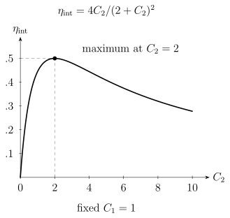
The two conversion paths must be balanced with the intermediate loss. This ideal resonant curve holds $C_1=1$ fixed. It does not include pump-dependent heating, external coupling losses, or added noise.

Zero excess photons does not mean zero loss

A simple phase-insensitive attenuator has

$$b_{\mathrm{out}} =\sqrt{\eta}\,e^{i\phi}a_{\mathrm{in}} +\sqrt{1-\eta}\,e,$$

where $e$ is an independent thermal environment mode with mean occupation $n_{\mathrm{th}}$. If added noise is defined as excess output photon number for a vacuum input, referred back to the signal input, then

$$n_{\mathrm{add}}=\frac{(1-\eta)n_{\mathrm{th}}}{\eta}, \qquad 0<\eta\leq1.$$

This normally ordered photon-number convention excludes vacuum’s half-quantum quadrature variance. Other noise conventions need conversion before comparison. Even when $n_{\mathrm{th}}=0$ and $n_{\mathrm{add}}=0$, loss replaces part of the signal by vacuum.

For example, restrict a pure-loss input to the single-rail qubit $\{|0\rangle,|1\rangle\}$. Its amplitude-damping Kraus operators are

$$\begin{aligned} K_0&=|0\rangle\langle0|+\sqrt\eta\,|1\rangle\langle1|,\\ K_1&=\sqrt{1-\eta}\,|0\rangle\langle1|. \end{aligned}$$

After correcting a known phase $\phi$, the Bloch-sphere-averaged fidelity to identity transfer is

$$F_{\mathrm{avg}}=\frac{3+2\sqrt\eta+\eta}{6}.$$

It equals only $1/2$ at complete loss. A dual-rail encoding instead puts the lost photon outside its one-photon code space, where an appropriate protocol can flag an erasure. Efficiency, noise, encoding, and heralding therefore belong in the same transfer model. Zeuthen et al. (2020) explains how conversion figures depend on the task; interconnects and transduction develops the channel perspective.

A longer memory lifetime must improve the intended storage task

A logical lifetime gain $G=\tau_L/\tau_{\mathrm{ref}}>1$ compares fitted decay times. The comparison must use the same state ensemble, metric, and physical reference. Encoding and decoding can introduce an initial cost. For example, suppose a common contrast-like measure is

$$Q_L(t)=A_L e^{-t/\tau_L},\qquad Q_{\mathrm{ref}}(t)=A_{\mathrm{ref}}e^{-t/\tau_{\mathrm{ref}}}.$$

If $\tau_L>\tau_{\mathrm{ref}}$ but $A_L<A_{\mathrm{ref}}$, the protected memory becomes better only after

$$t_*=\frac{\ln(A_{\mathrm{ref}}/A_L)} {1/\tau_{\mathrm{ref}}-1/\tau_L}.$$

A larger lifetime can therefore coexist with worse performance at short storage times. If the experimental metric has a nonzero asymptote, that baseline must first be handled consistently; the expression above is for the decaying contrast.

For a fixed, trace-preserving qubit channel, averaging state fidelity equally over the six Pauli eigenstates gives exactly the uniform Bloch-sphere average. This follows because their first and second Bloch moments match the sphere. It is not necessary to sample infinitely many input states. Unequal preparation errors, input-dependent acceptance, or nonlinear normalization after postselection invalidate that simple identification. Higher-dimensional encodings require the appropriate state ensemble.

Cat, binomial, and GKP encodings respond differently to photon loss, dephasing, ancilla faults, and imperfect control. Storage improvement does not alone establish protected logical gates. Blais et al. (2021) reviews circuit control and oscillator encodings; bosonic qubits explains the code and logical-operation requirements.

Exercises

1. High cooperativity without a split pair of poles

Set $g=1$, $\kappa=100$, $\gamma=0.01$, and $\gamma_\phi=0$, in common inverse-time units, at resonance. Find $C$ and determine whether the two poles have distinct real parts.

Solution

$C=4$. But $\gamma_\perp=0.005$, so the square-root argument is

$$1-\frac14(50-0.005)^2\simeq-623.875.$$

The square root is imaginary; both poles have real part $\omega_0$. Large cooperativity can arise from a very small noncavity decay rate without making the cavity coherent enough for repeated exchange.

2. Collection and propagation delay

An emitter has $\beta=0.92$ and $\Gamma_R:\Gamma_L=9:1$. Find the rightward fraction of all emitted photons. Separately, coupling points are $0.50\,\mathrm m$ apart in a guide with $v_g=0.40c$. For $\Gamma=2\pi(50\times10^6)\,\mathrm{s}^{-1}$, find $\Gamma\tau$.

Solution

$\mathcal D=(9-1)/(9+1)=0.8$ and the rightward fraction is $0.92(0.9)=0.828$. Leftward and nonguided fractions are $0.092$ and $0.08$.

Using $c\simeq3.0\times10^8\,\mathrm{m/s}$ gives $\tau\simeq4.17\,\mathrm{ns}$ and $\Gamma\tau\simeq1.31$. The envelope can change appreciably before a signal returns, so ignoring the propagation delay requires more than a reservoir label. The supplied $\Gamma$ is the coefficient in an exponential decay; quoting it divided by $2\pi$ does not change that definition.

3. An efficient internal converter can still lose the qubit

Take $C_1=C_2=10$, $\zeta_1=0.8$, $\zeta_2=0.7$, and no path loss. Find $\eta_{\mathrm{int}}$, $\eta$, and the average single-rail transfer fidelity if the only noise is pure loss. At fixed $C_1=10$, where is the internal conversion optimum?

Solution

$$\eta_{\mathrm{int}}=\frac{400}{441}\simeq0.9070,\qquad \eta=0.56\,\eta_{\mathrm{int}}\simeq0.5079.$$

Even with zero excess thermal photons,

$$F_{\mathrm{avg}} =\frac{3+2\sqrt{0.5079}+0.5079}{6}\simeq0.8222.$$

At fixed $C_1$, the optimum is $C_2=11$, with $\eta_{\mathrm{int,max}}=10/11\simeq0.9091$. The small internal improvement does not remove the external losses.

4. Lifetime gain and storage-time crossover

Take $\tau_L=2\,\mathrm{ms}$, $\tau_{\mathrm{ref}}=1\,\mathrm{ms}$, $A_L=0.90$, and $A_{\mathrm{ref}}=0.99$. Find the lifetime gain and the time after which the protected memory gives larger contrast.

Solution

$G=2$, while

$$t_*=\frac{\ln(0.99/0.90)}{1-1/2}\,\mathrm{ms} \simeq0.1906\,\mathrm{ms}.$$

The reference is better at shorter times in this model. The protected memory is better at longer times because its slower decay eventually compensates for encoding and decoding cost. A fitted lifetime by itself does not specify the better choice for a particular waiting time.

References

• Blais, A., Grimsmo, A. L., Girvin, S. M., and Wallraff, A. “Circuit Quantum Electrodynamics.” Reviews of Modern Physics 93, 025005 (2021). DOI: 10.1103/RevModPhys.93.025005.
• Kockum, A. F., Miranowicz, A., De Liberato, S., Savasta, S., and Nori, F. “Ultrastrong Coupling between Light and Matter.” Nature Reviews Physics 1, 19–40 (2019). DOI: 10.1038/s42254-018-0006-2.
• Zeuthen, E., Schliesser, A., Sørensen, A. S., and Taylor, J. M. “Figures of Merit for Quantum Transducers.” Quantum Science and Technology 5, 034009 (2020). DOI: 10.1088/2058-9565/ab8962.