Ultracold Atom Quantum Simulation

Ultracold atoms can reproduce the interactions and motion of useful quantum models in a setting where trapping, geometry, and measurement are tunable. The connection to the model depends on three physical questions: which Hamiltonian describes the atoms, which state was prepared, and what the detector actually measures. A low temperature or a detailed image answers only part of that problem.

This page develops those connections for lattice gases, synthetic fluxes, gauge constraints, and relaxation experiments. For dated results and open research questions, see Analog quantum simulation.

Required background. Ultracold atoms introduces degeneracy and collisions; optical lattices explains bands and localized orbitals. The Hubbard model and Bose–Hubbard model provide the many-body Hamiltonians.

Atomic motion becomes a lattice Hamiltonian

At sufficiently low energy, an atom in a deep periodic potential can be described using a localized orbital on each site. For two fermionic components, a common effective Hamiltonian is

$$H={}-\sum_{\langle i,j\rangle,\sigma} \left(t_{ij}c^\dagger_{i\sigma}c_{j\sigma} +t_{ij}^*c^\dagger_{j\sigma}c_{i\sigma}\right) +U\sum_i n_{i\uparrow}n_{i\downarrow} +\sum_{i,\sigma}V_i n_{i\sigma}.$$

Each undirected bond is counted once. The hopping amplitudes $t_{ij}$, onsite interaction $U$, and trapping offsets $V_i$ have units of energy. The complex conjugate in the reverse hopping is necessary when an artificial gauge field makes $t_{ij}$ complex. A chemical-potential term is added when an ensemble or reservoir requires it.

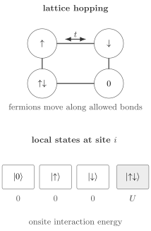
Hopping changes the occupation pattern. The onsite interaction distinguishes a doublon, containing both spin components, from an empty or singly occupied site. The indicated $U$ is the interaction contribution; trapping offsets and chemical potentials can add other local energies.

This description assumes that higher bands and other internal states can be neglected or eliminated consistently. Longer-range hopping, density-dependent hopping, finite-range interactions, and loss may need to be retained. Bloch, Dalibard, and Zwerger (2008) review how atomic parameters enter the effective models.

Eliminating a high-energy state is more than deleting its row and column from the Hamiltonian. Virtual visits to that state shift energies and generate couplings within the retained subspace. For example, in the half-filled repulsive Hubbard model at $U\gg|t|$, virtual doublons generate the antiferromagnetic exchange scale

$$J\simeq\frac{4|t|^2}{U}.$$

A bare projection that removes every doublon without keeping these virtual processes would miss the exchange. Effective Hamiltonians explains the systematic reduction. States and observables must be transformed consistently with the effective Hamiltonian.

Temperature must be compared with the relevant energy

Suppose a lattice has $U/|t|=8$. Then $J\simeq|t|/2$, so a temperature with $k_BT/|t|=0.5$ is already of order $J$. It may be low compared with the onsite interaction but too high for strong long-distance magnetic correlations. Lowering the tunnelling energy while keeping the same kelvin temperature can actually make the gas hotter in these dimensionless units.

Useful coordinates are $U/|t|$, $k_BT/|t|$, $k_BT/J$, filling, geometry, and trapping inhomogeneity. For the two-component one-orbital Hubbard model, half filling means one particle per site; hole doping is $\delta=1-\langle n_i\rangle$ in a homogeneous region. A single trapped cloud can contain several densities and therefore several local regimes.

Low $k_BT/J$ does not alone establish magnetic order. In the two-dimensional short-range SU(2)-symmetric model, continuous spin symmetry cannot be spontaneously broken at nonzero temperature in the thermodynamic limit. A finite cold cloud can nevertheless have a correlation length larger than its size and show strong staggered correlations. The distinction between finite-cloud ordering and a thermodynamic transition matters.

A thermometer compares measurements with a model

Lattice temperatures are commonly inferred from density fluctuations, spin correlations, response, or comparison with an independently characterized reservoir. Each inference assumes an equilibrium state and a suitable theoretical description. Uncertainty in hopping, interaction, filling, and detection can affect the inferred temperature together.

Several observables with different parameter dependence help distinguish temperature from other changes. For example, weaker antiferromagnetic correlations can result from higher temperature, doping, finite size, or an altered Hamiltonian. Fitting one correlator while holding all other parameters fixed can conceal these alternatives.

Determinant quantum Monte Carlo provides controlled benchmarks for the usual repulsive Hubbard model with real bipartite hopping at half filling. Doping, frustration, or additional terms can remove the symmetry that avoids the sign problem. Approximate methods remain useful, but their assumptions become part of the temperature inference. A fitted effective temperature in a nonequilibrium state need not describe every observable.

A microscope records measurement outcomes

A site-resolved image samples occupations or spins through a physical detection process. It is not a direct picture of a many-body wavefunction. The available outcomes depend on fluorescence, spin removal, atom loss, and whether multiple atoms can be distinguished. Gross and Bakr (2021) review these measurement possibilities.

For true binary occupation $n\in\{0,1\}$, let $\alpha$ be the probability of reporting empty when occupied, and $\beta$ the probability of reporting occupied when empty. If $p=\Pr(n=1)$,

$$p_{\rm obs}=\beta+(1-\alpha-\beta)p.$$

When $1-\alpha-\beta\ne0$, the mean can be inverted:

$$p=\frac{p_{\rm obs}-\beta}{1-\alpha-\beta}.$$

Near a zero denominator, small calibration and sampling errors are strongly amplified. At exactly zero, this detector carries no information about the binary occupation. Inverting noisy counts can also yield an unphysical estimate outside $[0,1]$; a likelihood model can enforce probability constraints while retaining calibration uncertainty.

Connected correlations need the joint channel

Let $m_i$ be the reported binary outcome and $a_i=1-\alpha_i-\beta_i$. If readout errors on different sites are independent conditional on the true occupations, then for $i\ne j$,

$$\operatorname{Cov}(m_i,m_j) =a_i a_j\,\operatorname{Cov}(n_i,n_j).$$

The offsets cancel in the connected covariance. This gives a useful correction under the stated factorization assumption. It does not follow from knowing only the corrected one-site means: the joint measured correlator is also needed. Correlated loss, hopping during imaging, or shared detection noise can add further terms.

Parity-sensitive detection is a different channel. If light-assisted collisions remove pairs, occupations $n=0$ and $n=2$ can both appear empty, while $n=1$ appears occupied. This is a many-to-one map, so a single parity image cannot distinguish a true hole from a doublon. Spin-resolved or number-resolved protocols provide additional information.

Synthetic flux is a phase around a closed loop

An internal-state label can play the role of a second lattice coordinate. Let $x$ be an integer real-space site index and $m$ an internal-state index. One possible hopping Hamiltonian is

$$H_{\rm syn}=-\sum_{x,m}\left[ t_x c^\dagger_{x+1,m}c_{x,m} +K_m e^{i\phi x}c^\dagger_{x,m+1}c_{x,m} +\mathrm{h.c.}\right].$$

Here $t_x$ and $K_m$ are energy amplitudes. If a resonant transition has angular Rabi frequency $\Omega_m$, its coupling magnitude is $|K_m|=\hbar|\Omega_m|/2$ under the usual two-level convention; the overall hopping sign can be included in its phase.

The phase of an individual link depends on basis choices. The product of link phases around an oriented plaquette is invariant under local changes of those basis phases. For a path that first moves in $+x$ and then in $+m$, the loop phase is $\phi$ modulo $2\pi$, as shown in Exercise 4. Reversing the path changes its sign.

The hopping graph resembles a two-dimensional lattice, but the interactions need not be local along the synthetic direction. Two internal states separated by many steps in $m$ can still occupy the same physical position. The measured internal-state populations are also unusually direct probes of synthetic edges.

A band invariant is not an occupation measurement

For an isolated Bloch band in two dimensions,

$$C=\frac{1}{2\pi}\int_{\rm BZ}\mathcal F_{xy}(\mathbf q)\,d^2q$$

is its Chern number, with $\mathcal F_{xy}$ the Berry curvature. The band does not have to be filled for this invariant to be defined. Filling, adiabaticity, interband transitions, and interactions enter the relation between the invariant and a measured Hall response or drift.

Cooper, Dalibard, and Spielman (2019) explain these links for cold atoms. A nonzero band Chern number alone does not establish an interacting fractional phase. Few-particle states, finite-system responses, and thermodynamic topological order require different interpretations. Particle-to-flux counting in a finite sample must also specify boundaries: an open $4\times4$ square lattice has nine elementary plaquettes, whereas the corresponding periodic lattice has sixteen. These are not interchangeable flux-counting geometries.

Gauge constraints are local conditions

A lattice gauge model specifies physical states by $G_j|\psi\rangle=g_j|\psi\rangle$ at every site. For fixed, dimensionless generators $G_j$, a useful mean squared deviation is

$$\epsilon_G=\frac1L\sum_j \left\langle(G_j-g_j)^2\right\rangle.$$

This quantity is nonnegative and cannot hide positive and negative violations by cancellation. Its numerical scale depends on the chosen generator normalization. A zero expectation of the signed sum of violations is a weaker condition, as Exercise 3 illustrates.

Constraint preservation and correct dynamics within the constrained space are separate. A large energy penalty can suppress transitions into unphysical states, but the surviving dynamics can still have incorrect couplings. Moreover, protection can slow a desired interaction when that interaction itself is generated through virtual intermediate states; it need not slow a target Hamiltonian that already acts directly within the physical space.

Finite-dimensional link models are useful quantum models in their own right. Relating them to a different link representation or a continuum gauge theory requires a separate truncation or continuum analysis. Halimeh et al. (2025) discuss the cold-atom implementations and their physical constraints.

Relaxation can preserve global purity

An isolated system evolves unitarily, so a pure global state remains pure. A subsystem can become mixed through entanglement with the rest:

$$\rho_A(\tau)=\operatorname{Tr}_B|\psi(\tau)\rangle\langle\psi(\tau)|, \qquad S_A=-\operatorname{Tr}\rho_A\ln\rho_A.$$

Subsystem entropy can therefore grow without increasing the total von Neumann entropy. Kaufman et al. (2016) measured this connection in an isolated atomic system. Entanglement growth by itself does not prove thermalization: integrable systems, constrained dynamics, and specially prepared states can approach different local descriptions.

Relaxation also need not be irreversible at every finite size or time. Dephasing can make observables approximately stationary over a useful window, while recurrences remain possible. A prethermal state can persist for a long interval before further relaxation or heating. A nonzero density imbalance over that interval shows retained memory; it does not by itself determine the infinite-time limit.

The detailed distinctions are developed in relaxation and thermalization, ETH, and many-body localization. For driven experiments, Floquet theory separates micromotion from evolution observed once per period.

Compare models through predictions for measured observables

The most informative calculation often predicts the actual experimental sequence: preparation, evolution, and readout. Comparing only a target ground state with an image can miss heating during a ramp or a detector that measures parity instead of number.

Small systems permit exact checks. Other regimes may be accessible to tensor networks, Monte Carlo, effective spin models, or controlled expansions. Their overlap helps identify the origin of discrepancies. A parameter inferred from one observable can then predict another, with the calibration uncertainty propagated.

Hamiltonian corrections and dissipative processes are mathematically different. For example, compare

$$\dot\rho=-\frac{i}{\hbar}[H_0+\delta H,\rho]$$

with

$$\dot\rho=-\frac{i}{\hbar}[H_0,\rho]+\mathcal D(\rho).$$

The dissipative superoperator $\mathcal D$ acts on density operators and cannot simply be added to a Hamiltonian. Similar-looking damping in one observable does not make the two models equivalent.

Near a phase boundary, over long times, or after a change of geometry, small omitted terms can become important. Agreement in a previously tested regime should therefore motivate specific predictions in the new regime, rather than imply that all larger-system results are already known. Analog simulation develops the general model correspondence and observable-error framework.

Exercises

1. Hubbard energy scales

A half-filled repulsive Hubbard simulator has

$$\frac{U}{t}=8, \qquad \frac{t}{h}=500\,\mathrm{Hz}, \qquad \frac{k_{\mathrm B}T}{t}=0.05.$$

1. Find $J/h$ for $J=4t^2/U$.
2. Find the superexchange time $h/J$.
3. Express the temperature as $k_{\mathrm B}T/J$ and as $k_{\mathrm B}T/h$.

Solution

Since $U=8t$,

$$J =\frac{4t^2}{8t} =\frac{t}{2}.$$

Therefore

$$\frac{J}{h} =250\,\mathrm{Hz}, \qquad \frac{h}{J} =4.0\,\mathrm{ms}.$$

The dimensionless temperature relative to exchange is

$$\frac{k_{\mathrm B}T}{J} = \frac{0.05t}{0.5t} =0.10,$$

and

$$\frac{k_{\mathrm B}T}{h} =0.05(500\,\mathrm{Hz}) =25\,\mathrm{Hz}.$$

The exercise shows why $k_{\mathrm B}T/t$ and $k_{\mathrm B}T/J$ answer different questions. Charge motion is measured against $t$, while the magnetic correlation scale is set by $J$. Here $h/J$ is one cycle of a relative phase at energy splitting $J$; the corresponding one-radian time is $\hbar/J$. The large-$U/t$ exchange formula is approximate.

2. Invert a microscope channel

A detector has false-negative probability $\alpha=0.03$ and false-positive probability $\beta=0.01$. It reports occupation probability $p_{\mathrm{obs}}=0.874$.

1. Invert the binary measurement model to find the true occupation $p$.
2. Why is the same scalar correction generally insufficient for a two-site connected correlator?

Solution

From

$$p_{\mathrm{obs}} =(1-\alpha)p+\beta(1-p),$$

we obtain

$$p = \frac{p_{\mathrm{obs}}-\beta} {1-\alpha-\beta} = \frac{0.874-0.01}{0.96} =0.900.$$

For a two-site correlator, the joint detector channel acts on four true outcomes. Correlated hopping or loss can make the two-site channel fail to factorize. Correcting each one-site mean and multiplying does not reconstruct $\langle n_i n_j\rangle$, so the connected quantity

$$\langle n_i n_j\rangle -\langle n_i\rangle\langle n_j\rangle$$

needs a calibrated joint or forward measurement model. If conditional readout errors do factorize and both sites have the specified error rates, the measured connected covariance is $0.96^2=0.9216$ times the true one.

3. Local versus global gauge checks

In an illustrative 71-constraint system, six local constraints have $G_j-g_j=\pm1$ for this one configuration, and all others satisfy the constraint exactly. Three violations are positive and three are negative.

1. Compute $\epsilon_G$.
2. Compute the mean signed violation.
3. Explain the diagnostic lesson.

Solution

Each violating site contributes one to the squared diagnostic:

$$\epsilon_G =\frac{6}{71} \approx 0.0845.$$

The signed mean is

$$\frac{1}{71} \sum_j(G_j-g_j) =\frac{3-3}{71} =0.$$

A global signed check would report perfect cancellation even though roughly $8.45\%$ of sites carry unit violations. Gauge symmetry is local, so the site-resolved distribution and its correlations are needed.

4. Flux in a synthetic plaquette

The hopping along a synthetic direction carries phase $e^{i\phi x}$, while real-direction hopping is real. Show that the phase accumulated around one real–synthetic plaquette is $\phi$. For $\phi=0.32\pi$, express the flux as a fraction of one flux quantum.

Solution

Traverse the plaquette from $(x,m)$ to $(x+1,m)$, then to $(x+1,m+1)$, back to $(x,m+1)$, and finally to $(x,m)$. The real hoppings contribute no phase. The forward synthetic hop contributes $e^{i\phi(x+1)}$ and the reverse synthetic hop contributes $e^{-i\phi x}$. Their product is

$$e^{i\phi(x+1)} e^{-i\phi x} =e^{i\phi}.$$

Thus the loop phase is $\phi$. Since one flux quantum corresponds to $2\pi$ phase,

$$\frac{\Phi}{\Phi_0} =\frac{\phi}{2\pi} =\frac{0.32\pi}{2\pi} =0.16.$$

The result identifies the single-particle Peierls flux. Interactions and finite synthetic width determine the many-body response.

5. Entanglement entropy is not by itself thermalization

Let a two-qubit pure state be $|\psi\rangle=(|00\rangle+|11\rangle)/\sqrt2$. Find the reduced state and entropy of A. Does this calculation show that a many-body system has thermalized?

Solution

Tracing out B gives $\rho_A=I/2$, whose entropy is $\ln2$. The full density matrix is a rank-one projector and has entropy zero. Thus local mixedness is compatible with global purity.

This one state does not demonstrate relaxation toward equilibrium. For a qubit Hamiltonian proportional to $Z$, $I/2$ is the infinite-temperature Gibbs state, but a thermal-looking reduced state at one instant does not establish a thermalization process or ETH. Dynamics, initial conditions, conserved quantities, and agreement of relevant observables with an ensemble must also be specified.

References

• Bloch, I., Dalibard, J., and Zwerger, W. “Many-body physics with ultracold gases.” Reviews of Modern Physics 80, 885–964 (2008). doi:10.1103/RevModPhys.80.885.
• Cooper, N. R., Dalibard, J., and Spielman, I. B. “Topological bands for ultracold atoms.” Reviews of Modern Physics 91, 015005 (2019). doi:10.1103/RevModPhys.91.015005.
• Gross, C., and Bakr, W. S. “Quantum gas microscopy for single atom and spin detection.” Nature Physics 17, 1316–1323 (2021). doi:10.1038/s41567-021-01370-5.
• Halimeh, J. C., Aidelsburger, M., Grusdt, F., Hauke, P., and Yang, B. “Cold-atom quantum simulators of gauge theories.” Nature Physics 21, 25–36 (2025). doi:10.1038/s41567-024-02721-8.
• Kaufman, A. M., Tai, M. E., Lukin, A., Rispoli, M., Schittko, R., Preiss, P. M., and Greiner, M. “Quantum thermalization through entanglement in an isolated many-body system.” Science 353, 794–800 (2016). doi:10.1126/science.aaf6725.