Attosecond Measurements and Ultrafast Dynamics

Ultrafast experiments use controlled light pulses to prepare and probe electronic and nuclear motion. They record spectra, photon counts, or particle momenta as a delay is varied. A physical model then connects those measurements to a pulse shape, a relative emission delay, or a changing molecular state.

The main distinctions are between pulse duration, experimental resolution, and precision in estimating a parameter. This page develops those distinctions and the assumptions behind common attosecond measurements. Dated experimental results and open questions are in Attosecond and ultrafast frontiers.

Required background. Ultrafast spectroscopy introduces pump–probe signals; photoelectron spectroscopy introduces ionization channels. Mode locking supplies the pulse language, and gauge choices explains why momentum and field conventions matter.

A short pulse needs bandwidth and controlled spectral phase

Let $E(t)$ be a square-integrable field envelope. Define rms temporal and angular-frequency widths using the normalized intensity distributions $|E(t)|^2$ and $|\widetilde E(\omega)|^2$. Fourier uncertainty gives

$$\sigma_t\sigma_\omega\geq\frac12.$$

For a transform-limited Gaussian, the intensity full widths at half maximum obey

$$\Delta t_{\mathrm{FWHM}}\Delta\nu_{\mathrm{FWHM}} =\frac{2\ln2}{\pi}\simeq0.441.$$

The widths must both use intensity and the same convention. Angular frequency is $\omega=2\pi\nu$. Mixing rms with FWHM widths, or frequency with angular frequency, produces large numerical errors.

Bandwidth alone does not fix duration. A spectral phase can delay different frequencies by different amounts without changing the spectrum. For a Gaussian spectrum with quadratic phase $\phi_2(\omega-\omega_0)^2/2$, the rms time width satisfies

$$\sigma_t^2=\frac1{4\sigma_\omega^2}+\phi_2^2\sigma_\omega^2.$$

Thus the transform-limited pulse is the shortest Gaussian with that spectrum. General spectral phases can also produce satellite pulses; one FWHM need not describe their full temporal extent.

The atomic unit of time is $\hbar/E_h\simeq24.19\,\mathrm{as}$. It is a unit derived from the Hartree energy, not a minimum possible duration or a literal orbit time. A stationary atomic state does not contain an electron following a classical orbit.

Resolution and fitted timing precision are different

For a weak-probe, time-invariant response model, a delay trace often has the form

$$S(\tau)=\int R(t)G(\tau-t)\,dt+\epsilon(\tau),$$

where $R$ is the physical response, $G$ the instrument response, and $\epsilon$ measurement noise. This convolution is an approximation; strong overlapping pulses can require a coherent nonlinear response calculation instead.

For independent Gaussian pump and probe timing profiles and Gaussian jitter, the corresponding rms widths add in quadrature:

$$\sigma_{\mathrm{IRF}}^2 =\sigma_{\mathrm{pump}}^2+\sigma_{\mathrm{probe}}^2 +\sigma_{\mathrm{jitter}}^2.$$

Geometry can supply another contribution if its distribution and independence are justified. Correlated timing fluctuations cannot simply be added as independent variances.

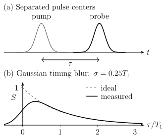
The lower plot convolves a causal exponential response with Gaussian timing blur of rms width $0.25T_1$. The apparent rise begins before nominal zero delay because of the instrument response; it is not a physical signal arriving before the excitation.

An identifiable parameter can nevertheless be estimated more precisely than the response width. For example, if $N$ independent photon arrival times follow a Gaussian of known width $\sigma$ and unknown center $t_0$, their sample mean has standard deviation $\sigma/\sqrt N$. For $\sigma=1\,\mathrm{fs}$ and $N=100$, this is $0.1\,\mathrm{fs}$. That does not mean arbitrary features separated by $0.1\,\mathrm{fs}$ can be resolved. Uncertain time zero, drift, and an incorrect response shape can also limit the estimate even when counting noise is small.

High harmonics combine electron motion and propagation

The gas-phase three-step model describes an electron released by a strong field, accelerated away from the ion, and driven back to recombine. For a linearly polarized monochromatic field $E(t)=E_0\cos\omega t$, its cycle-averaged quiver energy is

$$U_p=\frac{e^2E_0^2}{4m_e\omega^2},$$

where $e>0$ is the elementary charge and $E_0$ is the peak electric-field amplitude. In the simple model of release with zero initial velocity and no ionic force during propagation, the largest return kinetic energy is about $3.17U_p$. The emitted photon then has the cutoff estimate

$$\hbar\Omega_{\mathrm{cut}}\simeq I_p+3.17U_p.$$

This is not a general cutoff law for solids, arbitrary waveforms, or strongly multielectron dynamics. Even in a gas, Coulomb forces, depletion, and propagation can change what is observed.

The Keldysh parameter

$$\gamma_K=\frac{\omega\sqrt{2m_eI_p}}{eE_0} =\sqrt{\frac{I_p}{2U_p}}$$

compares the field timescale with a tunnelling scale. Small and large values organize tunnelling-like and multiphoton-like limits; the crossover is not a sharp boundary. A small value alone does not guarantee a valid quasistatic tunnelling formula, particularly near or above barrier suppression.

Emission from different positions interferes

For uniform source strength, constant phase mismatch $\Delta k$, no absorption, and a one-dimensional medium of length $L$,

$$E_{\mathrm{out}}\propto\int_0^L e^{i\Delta k z}\,dz, \qquad I_{\mathrm{out}}\propto L^2\operatorname{sinc}^2\!\left(\frac{\Delta kL}{2}\right),$$

where $\operatorname{sinc}x=\sin x/x$. At fixed nonzero mismatch, the buildup first vanishes at $L=2\pi/|\Delta k|$. More emitters can therefore give less detected light when their phases cancel.

Dispersion, focusing, plasma formation, and the microscopic dipole phase contribute to the mismatch. Absorption adds attenuation rather than simply another real phase. Short and long recollision contributions can also have different energy-dependent phases, producing an emission-time variation called attochirp. A high cutoff and a broad spectrum do not guarantee a short isolated pulse.

Krausz and Ivanov (2009) connects the source physics to ultrafast measurements. For the scattering approximations, see WKB and photoelectron spectroscopy.

Streaking maps a field into a momentum shift

Fix SI conventions with $\mathbf E=-\partial_t\mathbf A$ and $\mathbf A(\infty)=0$. Let a particle of charge $q$ be released at $t_i$ with kinetic momentum $\mathbf p_0$. Neglect the ionic force, magnetic force, and spatial field variation after release. Integrating the Lorentz force gives

$$\begin{aligned} \mathbf p_f-\mathbf p_0 &=q\int_{t_i}^{\infty}\mathbf E(t)\,dt\\ &=q\mathbf A(t_i). \end{aligned}$$

For an electron, $q=-e$, so

$$\mathbf p_f\simeq\mathbf p_0-e\mathbf A(t_i).$$

This sign follows from the stated definitions. The canonical momentum is $\mathbf p_{\mathrm{can}}=\mathbf p_{\mathrm{kin}}+q\mathbf A$; it is not the initially specified $\mathbf p_0$. Confusing the two momenta can reverse or double-count the streaking shift.

A real pulse releases amplitudes over a time interval, and the ion’s Coulomb force acts while the laser is present. A streaking spectrogram therefore contains more than a copy of the vector potential. Retrieval uses a forward model for ionization, continuum propagation, pulse phase, and detection. Pazourek, Nagele, and Burgdörfer (2015) reviews how those contributions affect inferred photoemission delays.

Two-path interferometry measures a relative phase

In RABBITT, a lower harmonic plus absorption of one infrared photon and an upper harmonic plus emission of one infrared photon reach the same photoelectron sideband. Choose the delay convention

$$\mathcal A(\tau)=A_+e^{i\omega\tau}+A_-e^{-i\omega\tau}.$$

Then

$$\begin{aligned} S(\tau)&=|A_+|^2+|A_-|^2 +2|A_+A_-|\cos(2\omega\tau-\Phi),\\ \Phi&=\arg A_--\arg A_+. \end{aligned}$$

Each amplitude includes the corresponding harmonic phase and a two-photon transition amplitude. The fitted $\Phi$ contains both. With this sign convention, a phase change $\Delta\Phi$ shifts a fixed fringe maximum by $\Delta\tau=\Delta\Phi/(2\omega)$. The phase is measured modulo $2\pi$, so interpreting a sequence of delays requires a reference and, when appropriate, phase unwrapping. Reversing the definition of positive delay reverses the corresponding reported sign.

A Wigner-like group delay is a spectral phase derivative, for example $\tau_W=\hbar\,\partial_E\arg d(E)$ for a specified transition amplitude and reference convention. The probe-induced continuum–continuum phase also contributes in a two-photon measurement. For long-range Coulomb potentials, an absolute free-flight comparison requires particular care; finite relative delays are usually the useful observables.

Many-electron correlation can already be included in $d(E)$ and hence in $\tau_W$. It should not be added once more as an independent “correlation delay.” Splitting a measured delay into scattering, probe, transport, and reference pieces is protocol dependent, with signs set by the reference subtraction. There is no universal sum of five independent positive delay times.

The outgoing electron can reduce ionic coherence

Suppose orthonormal ionic states $|I_j\rangle$ are correlated with normalized photoelectron packets $|e_j\rangle$:

$$|\Psi\rangle=\sum_j c_j|I_j\rangle|e_j\rangle, \qquad \sum_j|c_j|^2=1.$$

If the electron is not observed, the ionic density matrix has entries

$$\rho^{(I)}_{jk}=c_jc_k^*\langle e_k|e_j\rangle.$$

The overlap determines how much coherence survives. Orthogonal packets carry perfectly distinguishable channel information and remove the off-diagonal element. Identical packets preserve the maximum coherence allowed by the populations. The total state can remain pure in either case.

Selecting a photoelectron outcome can prepare a different conditional ionic state. Such conditioning does not restore the same coherence to the unselected ensemble. Nuclear motion, molecular orientation, and unobserved channels supply additional correlations in an actual experiment. Koll et al. (2026) demonstrates the relevance of ion–photoelectron entanglement to controlled ionic coherence in molecular photoionization.

A time-dependent hole density is consequently a reduced description. It need not determine the full molecular wavefunction. Likewise, under a suitable nonresonant, sufficiently energy-integrated scattering approximation, a signal can involve $\langle\rho^\dagger(\mathbf q)\rho(\mathbf q)\rangle$. Restricting to a coherent elastic contribution instead involves a squared mean amplitude, $|\langle\rho(\mathbf q)\rangle|^2$. These are not interchangeable. Energy acceptance, scattering channel, and sample averaging decide which model applies.

For the electron–nuclear dynamics, continue with nonadiabatic coupling and conical intersections. For deliberately changing a later molecular outcome, see molecular control.

Exercises

1. Bandwidth and timing

Find the minimum intensity FWHM energy bandwidth of a transform-limited Gaussian pulse of duration $100\,\mathrm{as}$, using $h=4.136\times10^{-15}\,\mathrm{eV\,s}$. Separately, Gaussian pump, probe, and independent jitter have rms widths $5.0$, $0.10$, and $0.30\,\mathrm{fs}$. Find the rms response width.

Solution

$$\Delta E=h\frac{0.441}{100\times10^{-18}\,\mathrm{s}} \simeq18.2\,\mathrm{eV}.$$

This assumes a transform-limited Gaussian. The separate timing example gives

$$\sigma_{\mathrm{IRF}} =\sqrt{5.0^2+0.10^2+0.30^2}\,\mathrm{fs} \simeq5.01\,\mathrm{fs}.$$

The pump dominates the preparation–probe resolution. A short probe does not erase the uncertainty in when the system was prepared.

2. Return energy and phase matching

An $800\,\mathrm{nm}$ monochromatic driver has $I=10^{14}\,\mathrm{W\,cm^{-2}}$ and the target has $I_p=15.76\,\mathrm{eV}$. Use $U_p[\mathrm{eV}]=9.337\times10^{-14} I[\mathrm{W\,cm^{-2}}]\lambda^2[\mu\mathrm m^2]$. Find $U_p$, $\gamma_K$, and the cutoff estimate. Why might a longer gas target fail to increase the signal?

Solution

$U_p\simeq5.98\,\mathrm{eV}$, $\gamma_K\simeq1.15$, and $I_p+3.17U_p\simeq34.7\,\mathrm{eV}$. The parameters lie near the multiphoton–tunnelling crossover.

At fixed nonzero mismatch, the uniform-medium amplitude cancels at $L=2\pi/|\Delta k|$. In a real target, absorption, focusing, depletion, and a changing plasma also affect buildup. The single-emitter cutoff and the macroscopic detected yield are different predictions.

3. Check the signs of two timing measurements

An electron is released where the vector potential points in the positive $x$ direction. Under the stated streaking assumptions, in which direction is its momentum kick? Separately, a RABBITT fringe phase increases by $0.60$ radians with infrared period $2.67\,\mathrm{fs}$. Find the shift of its maxima in the convention above.

Solution

The electron has $q=-e$, so $\Delta p_x=-eA_x<0$. This follows from integrating the force and does not depend on a mnemonic about the vector potential.

For the interferometric fringe,

$$\Delta\tau=\frac{\Delta\Phi\,T}{4\pi} =\frac{(0.60)(2.67)}{4\pi}\,\mathrm{fs} \simeq0.127\,\mathrm{fs}=127\,\mathrm{as}.$$

It is a positive shift in the chosen delay coordinate. Without a reference and separation of the optical and transition phases, it is not an isolated intrinsic emission delay.

4. A pure total state and a mixed ion

Take two equal ionic amplitudes and $\langle e_2|e_1\rangle=0.30e^{i\chi}$. Find $|\rho^{(I)}_{12}|$, the ionic purity, and its two eigenvalues.

Solution

The diagonal entries are $1/2$, and $|\rho^{(I)}_{12}|=0.15$. The eigenvalues are $(1\pm0.30)/2$, namely $0.65$ and $0.35$. Thus

$$\operatorname{Tr}[(\rho^{(I)})^2]=0.65^2+0.35^2=0.545.$$

Identical electron packets would give eigenvalues $1,0$ and purity one. Orthogonal packets would give $1/2,1/2$ and purity $1/2$. The mixedness comes from tracing over an entangled electron, not from assuming that the total state has become mixed.

References

• Koll, L.-M., et al. “Entanglement and Electronic Coherence in Attosecond Molecular Photoionization.” Nature 652, 82–88 (2026). DOI: 10.1038/s41586-026-10230-2.
• Krausz, F., and Ivanov, M. “Attosecond Physics.” Reviews of Modern Physics 81, 163–234 (2009). DOI: 10.1103/RevModPhys.81.163.
• Pazourek, R., Nagele, S., and Burgdörfer, J. “Attosecond Chronoscopy of Photoemission.” Reviews of Modern Physics 87, 765–802 (2015). DOI: 10.1103/RevModPhys.87.765.