Fundamental Symmetry Frontiers

Atoms and molecules can turn a very weak interaction into an accumulated phase or a small change in a transition probability. The experiment first measures that phase, frequency, or count asymmetry. Interpreting it as an electric dipole moment, a weak charge, or a new force then requires a calculated response of the particular system.

This page explains how symmetry signatures and complementary measurements connect those two steps. It develops the physical interpretation of the measurements rather than a ranking of current limits. Dated results and open questions are in Precision AMO tests.

Required background. Tests of fundamental symmetries introduces the measurement methods; Precision molecular measurements explains molecular response coefficients; Time reversal defines the antiunitary symmetry operation.

Spin-aligned electric dipole moments

For an isolated angular-momentum multiplet with no opposite-parity degeneracy, a permanent vector dipole can be parameterized as $\mathbf d=d\mathbf J/(J\hbar)$, where $J>0$ is the angular-momentum quantum number. In a weak external electric field its interaction is

$$H_d=-\frac{d}{J\hbar}\mathbf J\cdot\mathbf E.$$

Angular momentum is an axial vector: parity leaves $\mathbf J$ unchanged and reverses $\mathbf E$. Time reversal reverses $\mathbf J$ and leaves $\mathbf E$ unchanged. The product $\mathbf J\cdot\mathbf E$ is therefore odd under both operations. A nonzero intrinsic coefficient $d$ describes parity- and time-reversal-violating physics.

This conclusion concerns an intrinsic spin-aligned dipole. An ordinary polar molecule can have a body-fixed electric dipole without violating either symmetry. An electric field mixes rotational parity states and orients that dipole in the laboratory. It supplies an external polar direction; the induced orientation is not the intrinsic spin-aligned coefficient above. Degenerate opposite-parity states and prepared superpositions require the same care about what fixes the direction.

Under CPT invariance, time-reversal violation implies CP violation. The assumptions are explained in Discrete symmetries and CPT. Chupp et al. (2019) review how EDM measurements connect to microscopic interactions.

A phase convention with an explicit factor of two

For a two-level sensor, define the effective Hamiltonian

$$H_s=-\left(\mu B+d\mathcal E\right)\sigma_z, \qquad \mathcal E=\mathcal P E_{\rm eff}.$$

Here $\mathcal P$ is a signed orientation factor and $E_{\rm eff}$ is the response coefficient in the chosen molecular convention. Define the signed splitting as $E_- -E_+$, with $\sigma_z|\pm\rangle=\pm|\pm\rangle$. The corresponding angular frequency is

$$\omega=\frac{2(\mu B+d\mathcal E)}{\hbar}, \qquad \phi=\omega\tau.$$

The factor of two follows from the two eigenvalues in this definition. Another choice of levels or response coefficient can absorb that factor; the observable must be translated with the same convention throughout. An effective molecular field is a coefficient relating the microscopic interaction to an energy shift, not simply the laboratory electrode field.

Reversing $\mathcal P$ changes the EDM term’s sign. It can also change an ordinary magnetic or light shift through imperfect control. A laboratory reversal selects a sign pattern; it does not perform the full antiunitary time-reversal transformation or uniquely identify the physical cause.

Which microscopic interaction was measured?

A molecular frequency can respond to several interactions:

$$\hbar\omega_i=K_{ie}d_e+K_{iS}C_S+\cdots.$$

The coefficients include the level splitting and orientation convention. $C_S$ can represent a scalar–pseudoscalar electron–nucleon interaction, with its normalization specified by the chosen effective Hamiltonian. One measurement restricts a combination of $d_e$ and $C_S$. A limit on $d_e$ alone usually assumes the other contributions vanish or are constrained independently.

Atomic and nuclear observables introduce further response calculations. For example, screening suppresses a pointlike nuclear EDM in an ideal neutral nonrelativistic electrostatic atom; finite nuclear size and other departures from those assumptions permit observable effects. A nuclear Schiff moment is one relevant finite-size quantity. Nuclear and electronic calculations are both needed to relate it to a measured atomic EDM. The detailed screening derivation is in Tests of fundamental symmetries.

The Standard Model already violates CP. Its weak-interaction contributions to many EDM observables are very small, but the strong interaction also allows the QCD $\bar\theta$ parameter, whose size is not predicted to be small merely by writing down the Standard Model. Thus an EDM observation would establish a nonzero P- and T-odd effect; deciding which microscopic source it requires needs its magnitude, the system responses, and other measurements. It would not by itself explain the cosmic matter asymmetry.

Reversals and ordinary backgrounds

For two binary switches $s,t=\pm1$, any four cell means can be written

$$f(s,t)=f_0+a s+b t+c st.$$

The interaction coefficient is exactly

$$c=\frac14\left[f(+,+)-f(+,-)-f(-,+)+f(-,-)\right].$$

The constant and single-switch terms cancel. If a nuisance shift also proportional to $st$ is present, however, it adds directly to $c$. Reversal algebra cannot separate two effects with the same sign pattern. An additional measurement or a controlled variation that changes their responses differently is needed.

Unequal repeat counts do not invalidate this formula when applied to the four unbiased cell means. They change its variance. A naive signed average over all individual shots, without accounting for unequal counts, generally does mix channels. A regression with the appropriate design matrix and noise covariance handles unequal sampling and calibrated drift terms. Missing switch states can make some coefficients unidentifiable.

For example, suppose a magnetic field correlated with electric-field reversal changes by $\delta B$. Its phase shift is proportional to $\mu\delta B$, which can mimic $d\mathcal E$. Changing the electric-field magnitude, using an internal molecular reversal, or measuring an auxiliary magnetic response can help distinguish them, provided the nuisance response to that change is also understood.

Complementary systems constrain different combinations

Write several measurements as

$$\mathbf y=K\mathbf c+\boldsymbol\epsilon, \qquad \operatorname{Cov}(\boldsymbol\epsilon)=\Sigma.$$

The vector $\mathbf c$ contains the interaction coefficients, and each row of $K$ describes one experiment’s response. For fixed known $K$, Gaussian noise, and an identifiable linear model, the least-squares covariance is

$$\operatorname{Cov}(\widehat{\mathbf c}) =\left(K^{\mathsf T}\Sigma^{-1}K\right)^{-1}.$$

Two very precise measurements can still leave a poorly constrained combination if their response rows point in almost the same direction. For coefficients expressed in fixed common units, compare

$$K_{\parallel}=\begin{pmatrix}1&1\\1&1.01\end{pmatrix}, \qquad K_{\perp}=\begin{pmatrix}1&1\\1&-1\end{pmatrix}.$$

The first pair measures almost the same sum twice. Its difference determines $0.01c_2$, amplifying the measurement noise when solving for $c_2$. The second pair directly measures a sum and a difference.

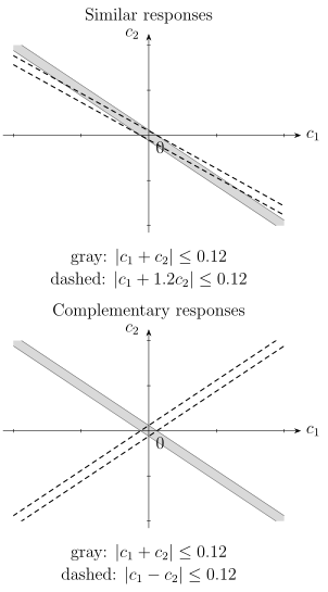
Each band represents values compatible with one hypothetical measurement. Nearly parallel bands leave a long allowed direction. A second response that crosses the first at a large angle can constrain both coefficients. For visibility, the upper dashed band uses $c_1+1.2c_2$ rather than the still closer response in $K_{\parallel}$. Axes use fixed illustrative coefficient units; these are not experimental exclusion limits.

Raw determinants and condition numbers depend on the units assigned to the coefficients. For quantitative comparisons, whiten the data with $\Sigma^{-1/2}$ and scale each coefficient by a stated physically relevant reference value. Singular values of that scaled response show which combinations are weakly measured. Rescaling units cannot create physical information.

Response uncertainty also matters. If a row of $K$ has covariance $\Sigma_K$, then, conditional on fixed $\mathbf c$, its contribution to the predicted observable variance is $\mathbf c^{\mathsf T}\Sigma_K\mathbf c$. It is generally parameter dependent, not a constant extra noise term. Correlated theory errors should be retained when combining systems that use related calculations. The global-fit approach is illustrated by Chupp and Ramsey-Musolf (2015).

Parity violation through interference

A weak interaction can mix opposite-parity atomic or molecular states. The resulting small transition amplitude can be measured through its interference with a controllable reference amplitude. If a switch changes the latter from $A_0$ to $-A_0$, while leaving $A_{\rm PV}$ fixed, then

$$R_\pm=|\pm A_0+A_{\rm PV}|^2, \qquad R_+-R_-=4\operatorname{Re}(A_0^*A_{\rm PV}).$$

This difference is linear in the small weak amplitude. The normalized asymmetry is

$$\frac{R_+-R_-}{R_++R_-} =\frac{2\operatorname{Re}(A_0^*A_{\rm PV})} {|A_0|^2+|A_{\rm PV}|^2}.$$

When $|A_{\rm PV}|\ll|A_0|$, the denominator can be approximated by $|A_0|^2$. But if the two amplitudes are exactly in quadrature, their real interference term vanishes. Simply adding a real Stark matrix element and an imaginary weak matrix element to a static two-level Hamiltonian does not guarantee a population signal linear in the weak interaction. The pulse timing, detuning, geometry, and measured quadrature determine whether the required relative phase is present.

The measured parity-violating amplitude is related to a weak charge or spin-dependent weak coefficient through atomic or molecular theory. At tree level, the nuclear weak charge has the approximate form $Q_W=-N+Z(1-4\sin^2\theta_W)$; precision use requires radiative and nuclear corrections. Isotope comparisons can reduce shared electronic uncertainty while retaining sensitivity to neutron distributions. Safronova et al. (2018) discuss these connections and the different AMO tests.

Isotope shifts and departures from King linearity

For transition $i$ and isotopes $A,A'$, define $\delta\nu_i^{AA'}=\nu_i^A-\nu_i^{A'}$ and $\mu^{AA'}=1/M_A-1/M_{A'}$. A leading mass-plus-field-shift model is

$$\delta\nu_i^{AA'}=K_i\mu^{AA'}+F_i\delta R^{AA'}, \qquad R_A=\langle r^2\rangle_A.$$

For nonzero $\mu$, divide by it to obtain the modified shift $m\nu_i=\delta\nu_i/\mu$. Eliminating $\delta R/\mu$ between transitions $i,j$, with $F_j\ne0$, gives

$$m\nu_i=\left(K_i-\frac{F_i}{F_j}K_j\right) +\frac{F_i}{F_j}m\nu_j.$$

The points lie on a line under this two-factor model. Higher nuclear moments, polarization, and higher-order mass or field shifts can add independent factors. A candidate new interaction can do so too, but only when its transition and isotope dependences are sufficiently independent of the included terms. Berengut and Delaunay (2025) explain this use of isotope-shift spectroscopy.

Higher-order shifts must remain isotope differences

An isotope shift is a difference of two transition frequencies. It is antisymmetric and additive:

$$\delta\nu^{AB}=-\delta\nu^{BA}, \qquad \delta\nu^{AB}+\delta\nu^{BC}=\delta\nu^{AC}.$$

A schematic smooth radius-dependent frequency can be expanded around one fixed reference isotope 0. Let $q_A=R_A-R_0$ and write its field-dependent part as $F_iq_A+G_iq_A^2$. Then

$$\delta\nu_i^{AB} =K_i\mu^{AB}+F_i(q_A-q_B)+G_i(q_A^2-q_B^2).$$

The last term is generally not $G_i(q_A-q_B)^2$. Squaring a pair difference would lose antisymmetry and fail the addition rule. Against the fixed reference 0, it does reduce to $G_iq_A^2$, because $q_0=0$. This illustrative expansion is not a claim that one quadratic radius term captures every higher-order nuclear effect.

Additional transitions and isotopes help separate candidate dependences, but do not guarantee that they are independent. A nonlinear King plot shows that the leading model is inadequate at the achieved precision; it does not uniquely specify which missing interaction or nuclear correction caused the deviation.

Static new forces and oscillating fields

A static exchanged boson of mass $m_b$ has characteristic range $\lambda_b=\hbar/(m_bc)$. A spin-independent Yukawa potential can be parameterized as

$$V(r)=\pm\frac{\hbar c\,g_1g_2}{4\pi r}e^{-r/\lambda_b},$$

where the sign and coupling normalization depend on the chosen microscopic interaction. A finite source requires integrating this kernel over its spatial density. A spin-dependent interaction also depends on the spin and possibly velocity geometry. The mediator’s name alone does not fix the parity or time-reversal character of the complete potential; the couplings and operator structure matter. Cong et al. (2025) provide the corresponding potential classifications.

An ambient oscillating field is a different source model. Its amplitude, frequency distribution, and coherence time depend on the assumed field population. A dark-matter interpretation includes an assumption about the fraction of local dark matter in that field. A laboratory force sourced by nearby matter does not require that abundance assumption.

The instrument measures a response to either source through its transfer function. A spectral peak at a source-modulation frequency can also come from magnetic leakage or mechanical motion. Changing source distance, polarization, or detector orientation tests specific spatial and angular predictions, while calibration at the measurement frequency connects the recorded amplitude to the proposed interaction.

Interpreting a null result

An interval containing zero means the data are compatible with zero under the stated model; it does not establish exact vanishing. A frequentist confidence level describes the repeated-sampling coverage of the interval procedure. A Bayesian credible level describes posterior probability under the specified likelihood and prior. These interpretations should not be interchanged.

The signed EDM coefficient can be positive or negative. The derived magnitude $|d|$ has a boundary at zero, so a limit on the magnitude needs an interval construction appropriate to that quantity. A projection-noise estimate alone is neither construction.

Likewise, converting a bound on $C/\Lambda^2$ into a lower bound on a heavy-particle scale $\Lambda$ requires a choice of coupling $C$, phases, operator content, and possible cancellations. Experiments measure low-energy responses; the particle-model interpretation adds those assumptions.

Exercises

An EDM phase in SI units

Use $d=10^{-30}\ e\,{\rm cm}$, $\mathcal E=23\ {\rm GV/cm}$, and $\tau=1\ {\rm s}$ in the two-level convention above. Find the EDM phase. For $N=10^6$ independent particles and contrast $C=0.80$, use a mid-fringe phase uncertainty $1/(C\sqrt N)$ to estimate the uncertainty in $d$.

Solution

Since $1\ e\,{\rm cm}=1.602176634\times10^{-21}\ {\rm C\,m}$, $d=1.602176634\times10^{-51}\ {\rm C\,m}$ and $\mathcal E=2.3\times10^{12}\ {\rm V/m}$. Thus $\phi_d=2d\mathcal E\tau/\hbar\simeq6.99\times10^{-5}$ radians. The idealized uncertainty is

$$\delta d=\frac{\hbar}{2C\mathcal E\tau\sqrt N} \simeq1.79\times10^{-29}\ e\,{\rm cm}.$$

This is a statistical scale for the stated ensemble and operating point. It omits additional noise, duty cycle, response uncertainty, and correlated systematic shifts; it is not a confidence limit.

Unequal sampling of reversal states

Let the four cell means for $(s,t)=(++,+-,-+,--)$ be $(13,9,5,13)$ Hz. Find $c$. If the repeat counts are $(2,1,1,1)$, compare with a naive signed average over all shots, treating each shot as equal to its cell mean for this illustration.

Solution

The cell-mean projection gives $c=(13-9-5+13)/4=3$ Hz. The naive shot average gives $(2\times13-9-5+13)/5=5$ Hz. It overweights the $++$ cell and no longer cancels the other channels. The correct projection remains valid for the four cell means; the repeat counts affect their precision and hence the estimator’s variance.

Two precise but similar responses

Assume independent unit-variance errors and known response matrix $K_\parallel$ above. Find $\operatorname{Var}(\widehat c_2)$ by subtracting the two measurements. Compare with $K_\perp$.

Solution

For $K_\parallel$, $\widehat c_2=(y_2-y_1)/0.01$, so its variance is $2/(0.01)^2=20000$. For $K_\perp$, $\widehat c_2=(y_1-y_2)/2$ and the variance is $2/4=0.5$. Both calculations use the same coefficient units and measurement variance. The improvement comes from independent response directions, not from changing the units of the parameters.

A quadratic isotope term

In fixed radius units let $q_A=2$, $q_B=1$, and $q_C=0$. Consider only the term $Gq^2$. Calculate its shifts for $AB$, $BC$, and $AC$ and verify addition. What goes wrong if one instead uses $G(q_A-q_B)^2$ for every pair?

Solution

The proper differences are $3G$, $G$, and $4G$, and $3G+G=4G$. The squared pair-difference rule gives $G$, $G$, and $4G$, failing addition. It also gives the same result after swapping $A$ and $B$, rather than the required opposite sign. The quadratic expansion is consistent when applied to each isotope’s frequency before taking the difference.

References

• Berengut, J. C., and C. Delaunay. “Precision isotope-shift spectroscopy for new physics searches and nuclear insights.” Nature Reviews Physics 7, 119–125 (2025). doi:10.1038/s42254-024-00793-2.
• Chupp, T. E., P. Fierlinger, M. J. Ramsey-Musolf, and J. T. Singh. “Electric dipole moments of atoms, molecules, nuclei, and particles.” Reviews of Modern Physics 91, 015001 (2019). doi:10.1103/RevModPhys.91.015001.
• Chupp, T., and M. Ramsey-Musolf. “Electric dipole moments: A global analysis.” Physical Review C 91, 035502 (2015). doi:10.1103/PhysRevC.91.035502.
• Cong, L., et al. “Spin-dependent exotic interactions.” Reviews of Modern Physics 97, 025005 (2025). doi:10.1103/RevModPhys.97.025005.
• Safronova, M. S., D. Budker, D. DeMille, D. F. Jackson Kimball, A. Derevianko, and C. W. Clark. “Search for new physics with atoms and molecules.” Reviews of Modern Physics 90, 025008 (2018). doi:10.1103/RevModPhys.90.025008.