Precision Molecular Measurements

A precision molecular measurement infers a small interaction from a resolved molecular frequency or accumulated quantum phase. Heavy atoms can provide a large electronic response, while closely spaced rotational or parity levels let modest laboratory fields control that response. The useful combination is a large, understood energy shift and a comparison that distinguishes it from ordinary magnetic, electric, and motional shifts.

This page develops the molecule as a sensor: orientation, electron and nuclear symmetry tests, chiral transitions, and the conversion from a measured phase to an interaction strength. Tests of Fundamental Symmetries develops the wider experimental comparison; Fundamental Symmetry Frontiers discusses research status.

Helpful background. Molecular Quantum Mechanics introduces molecular energy scales, Rotations of Molecules develops angular states and Stark mixing, and Precision Spectroscopy explains frequency estimation.

Molecular energy shifts and response coefficients

Let $c_i$ be small interaction coefficients and let channel $a$ compare states $u_a$ and $l_a$. Define the complete laboratory response

$$K_{ai}=\left. \frac{\partial(E_{u_a}-E_{l_a})}{\partial c_i} \right|_{\mathbf c=0}.$$

The derivative includes the actual field-dressed states, their angular factors, and the difference between the two levels. To first order,

$$y_a\equiv h\,\delta\nu_a =\sum_i K_{ai}c_i+\sum_j A_{aj}\eta_j+\epsilon_a.$$

Here $\eta_j$ describes an unwanted but modeled effect, such as a magnetic field correlated with an electric-field reversal; $A_{aj}$ converts it to an energy. The noise vector $\boldsymbol\epsilon$ has covariance $\Sigma$. If a calculation instead supplies a body-fixed coefficient $W_i$, its angular factor must be included when constructing $K_{ai}$. Multiplying an already complete derivative by another polarization factor counts the same state mixing twice. Different operators need not share one factor.

This distinction also explains why a molecule has several sensitivities. A state useful for the electron electric dipole moment need not be equally useful for a nuclear Schiff moment. The relevant electronic operator, nuclear spin, angular matrix element, and coherence time all matter.

What can several measurements determine?

In matrix form, $\mathbf y=K\mathbf c+A\boldsymbol\eta+\boldsymbol\epsilon$. With known nuisances, the rank of $K$ counts independently accessible coefficient combinations. With unknown nuisances, some of those combinations can be indistinguishable from an ordinary shift.

For Gaussian noise and freely fitted nuisances, whiten the data using $\widetilde K=\Sigma^{-1/2}K$ and $\widetilde A=\Sigma^{-1/2}A$. If $\widetilde A$ has independent columns, the information remaining about $\mathbf c$ is

$$\begin{aligned} F_c&=\widetilde K^{\mathsf T}P_\perp\widetilde K,\\ P_\perp&=I-\widetilde A (\widetilde A^{\mathsf T}\widetilde A)^{-1} \widetilde A^{\mathsf T}. \end{aligned}$$

The projection removes changes that a nuisance could reproduce. For dependent nuisance columns, use the orthogonal projector onto their column space, for example through a singular-value decomposition. Independent calibration or a stated prior can recover information; assuming a nuisance is zero cannot substitute for that measurement. Fisher Information explains the statistical construction. Exercises 4 and 8 give small examples.

Parity doublets and laboratory orientation

A polar molecule has a body-fixed electric dipole $\mathbf D=D\hat{\mathbf n}$, with a directed molecular axis $\hat{\mathbf n}$. Nevertheless, a field-free parity eigenstate has $\langle\hat{\mathbf n}\rangle=0$: its orientation distribution is unchanged under $\hat{\mathbf n}\mapsto-\hat{\mathbf n}$. A polar bond and a nonzero laboratory mean dipole are different statements.

Take two opposite-parity levels separated by an energy $\Delta_P>0$. Choose their relative phase so that the laboratory dipole matrix element $d_p=|\langle+|D_z|-\rangle|$ is positive. In this two-state subspace,

$$H=\frac{\Delta_P}{2}\sigma_z-d_p\mathcal E\sigma_x, \qquad D_z=d_p\sigma_x,$$

where $\mathcal E$ is the signed electric field along $z$. Diagonalization and the Hellmann–Feynman theorem give

$$\begin{aligned} E_\pm&=\pm\frac12\sqrt{\Delta_P^2+4d_p^2\mathcal E^2},\\ \langle D_z\rangle_-&=-\frac{\partial E_-}{\partial\mathcal E} =d_p\frac{x}{\sqrt{1+x^2}}, \qquad x=\frac{2d_p\mathcal E}{\Delta_P}. \end{aligned}$$

The signed doublet mixing fraction is $p=x/\sqrt{1+x^2}$. It is linear in weak field and approaches $\pm1$ when the Stark coupling greatly exceeds the doublet splitting. But the geometric orientation relative to the body-fixed dipole is

$$\mathcal P_z\equiv\langle n_z\rangle =\frac{d_p}{D}\,p.$$

Usually $d_p\ne D$. For an ideal Hund-case-(a) doublet at fixed $J,M$ and $|\Omega|$, neglecting hyperfine and other rotational-level mixing, $d_p/D=|M\Omega|/[J(J+1)]$. Thus $J=M=|\Omega|=1$ gives $|\mathcal P_z|\to1/2$ even when $|p|\to1$. The molecule still has rotational angular spread. Stronger fields that mix other $J$ levels require a larger Hamiltonian and can change this limiting orientation. Brown and Carrington develop these angular matrix elements; Hutzler explains the role of small parity splittings in molecular sensing.

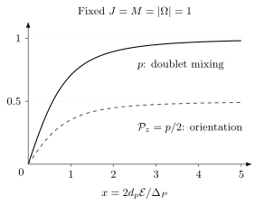
Complete mixing of a parity doublet does not mean a sharply aligned molecular axis. The solid curve is $p=x/\sqrt{1+x^2}$; the dashed curve is $\mathcal P_z=p/2$ for the stated fixed-$J$ example. Both curves assume other rotational and hyperfine states can be neglected.

The field required for strong doublet mixing scales with $\Delta_P/d_p$. This small energy denominator controls orientation; a separate electronic matrix element controls the response to a microscopic interaction. Hyperfine structure, nearby levels, and field-dependent magnetic moments must be included when they affect the intended accuracy.

Electron electric dipole moments and Ramsey phases

The electron electric dipole moment $d_e$ couples through a relativistic operator. A molecular effective electric field summarizes its matrix element. It is a calculated response coefficient, not the applied electrode field or a classical field to insert into an unrelated Stark Hamiltonian. Relativistic electronic structure near a heavy nucleus can make this coefficient large; bonding and electron correlation still matter quantitatively.

To fix all factors, label two measured states $a,b$ and choose the order of their energy difference so that

$$\Delta E_{ab}^{(d_e)}=2\eta_d d_eE_{\rm eff}, \qquad \phi_{d_e}=\frac{2\eta_d d_eE_{\rm eff}\tau}{\hbar}.$$

Here $E_{\rm eff}>0$ is the magnitude of the fully polarized single-state response, and $\eta_d$ is the signed response reduction for this pair; the chosen fully polarized reference has $\eta_d=1$. Calculate $\eta_d$ from the EDM operator in the actual states. It can equal a doublet mixing fraction in a simple model, but is not generally the geometric $\langle n_z\rangle$.

Another common convention uses a body-fixed coefficient $W_d$ with single-state shift $d_eW_d\Omega$, where $\Omega$ is dimensionless. In that convention the fully polarized magnitude is $E_{\rm eff}=|W_d\Omega|$. Do not multiply this $E_{\rm eff}$ by an additional $\Omega$. An ordinary frequency is $\Delta E/h$, whereas a phase accumulation rate is $\Delta E/\hbar$.

Competing operators and historical examples

Paramagnetic molecules can also respond to a scalar electron–nucleon coupling $C_S$. A pair channel can therefore take the form

$$h\,\delta\nu=K_d d_e+K_S C_S+\cdots.$$

One measured channel constrains a combination. A limit on $d_e$ obtained by setting $C_S=0$ is a conditional, single-source limit. Several molecules help separate operators when their response rows are sufficiently different, after accounting for experimental and theory correlations. Chupp and collaborators review this interpretation.

As a concrete historical example, Roussy and collaborators reported in 2023 an HfF$^+$ result

$$d_e=(-1.3\pm2.0_{\rm stat}\pm0.6_{\rm syst}) \times10^{-30}\ e\,{\rm cm},$$

with $|d_e|<4.1\times10^{-30}\ e\,{\rm cm}$ at 90% confidence under the single-source interpretation. Their trapped-ion measurement used coherence times up to about $3\ {\rm s}$ and an effective field near $23\ {\rm GV\,cm^{-1}}$. The 2018 ACME ThO beam measurement reported $|d_e|<1.1\times10^{-29}\ e\,{\rm cm}$ at 90% confidence, illustrating a different experimental architecture. These dated examples explain the measurement scales; current comparisons belong in the linked frontier discussion.

Reversals separate shifts with different symmetries

A Ramsey experiment prepares a superposition, lets its phase evolve, and converts the phase into a population difference. Repeating this sequence under binary switches $s_q=\pm1$ gives the expansion

$$f(\mathbf s)=\sum_S f^S\prod_{q\in S}s_q.$$

Balanced averages isolate the coefficient with the expected signal parity. An ordinary shift with the same switch dependence is not removed by this algebra. For example, if the unwanted pair magnetic energy is $\Delta E_B=2\mu_{\rm eff}B_{\rm corr}$, its equivalent EDM is

$$d_{\rm false}=\frac{\mu_{\rm eff}B_{\rm corr}} {\eta_d E_{\rm eff}}.$$

Both numerator and denominator now use the same pair convention. Field measurements and deliberately exaggerated magnetic correlations test this leakage. Actual field magnitudes also matter: a commanded reversal can change the magnitude and thereby convert an ordinary Stark shift into a switch-dependent signal.

Nearby internal states can reverse the microscopic response while sharing much of the magnetic environment. This internal comagnetometer suppresses common shifts, but differences in $g$ factors, Stark shifts, trajectories, and detection efficiency remain measurable limitations. Geometric phases arise when moving molecules follow changing field directions; varying field rotation or molecular motion tests their contribution. Conditioning on survival can also bias a comparison if loss differs between switch states.

Nuclear symmetry tests in molecules

Electronic wavefunctions near a heavy nucleus convert nuclear interactions into spectroscopic shifts. Several distinct nuclear quantities can be probed; their angular responses must not be interchanged.

Schiff moments and screening

In a stationary neutral bound system of nonrelativistic point charges with electrostatic interactions, the leading effect of a point nuclear EDM is screened. Real nuclei have finite size, and magnetic and relativistic effects need separate treatment. Ions also require a modified screening analysis. Schiff’s theorem therefore does not remove all nuclear $P,T$-odd effects (Schiff; Flambaum and Kozlov).

A finite-size source is the nuclear Schiff moment $\mathcal S$. For a nucleus with $I\ne0$, a schematic molecular interaction is

$$H_{\mathcal S}=W_{\mathcal S}\mathcal S \frac{\mathbf I\cdot\hat{\mathbf n}}{I}.$$

Here $\mathbf I$ is a dimensionless spin operator, with $\mathbf I^2=I(I+1)$; $W_{\mathcal S}\mathcal S$ has energy units. The normalization of $\mathcal S$ and its sign convention must match the electronic calculation. Inferring a Schiff moment from a frequency needs that electronic response; inferring underlying nuclear or hadronic couplings needs additional nuclear theory.

Octupole-correlated nuclei can have nearby opposite-parity states. For an initially positive-parity state, first-order mixing gives

$$\langle\widehat{\mathcal S}\rangle \simeq2\operatorname{Re} \frac{\langle+|\widehat{\mathcal S}|-\rangle \langle-|V_{P,T}|+\rangle}{E_+-E_-}.$$

The small denominator can enhance the response, provided $|\langle-|V_{P,T}|+\rangle|\ll|E_+-E_-|$. At a degeneracy one must diagonalize the coupled states; the first-order expression cannot grow without limit. Nuclear matrix elements and correlations are as important as the energy separation (Dobaczewski and collaborators).

Magnetic quadrupoles and spin-dependent parity violation

A nuclear magnetic quadrupole moment $\mathcal M$ requires $I\ge1$ and couples through a rank-two angular operator, schematically $H_{\mathcal M}=W_{\mathcal M}\mathcal M\Xi_{\mathcal M}$. The dimensionless $\Xi_{\mathcal M}$ depends on the molecular electronic and hyperfine states. It cannot be replaced by the rank-one Schiff angular factor.

Nuclear-spin-dependent parity violation is a different interaction. In relativistic units $\hbar=c=1$, a common convention for a selected nucleus with $I\ne0$ is

$$H_{\rm NSD}=\frac{G_F}{\sqrt2}\kappa_{\rm NSD} \sum_e\rho_N(\mathbf r_e)\, \boldsymbol\alpha_e\cdot\frac{\mathbf I}{I}, \qquad \int\rho_N(\mathbf r)\,d^3r=1.$$

$\boldsymbol\alpha_e$ acts on electron $e$ and $G_F$ is the Fermi constant in these units. Nuclear anapole, weak neutral-current, and weak–hyperfine contributions can enter $\kappa_{\rm NSD}$, with convention-dependent factors. The perturbation mixes opposite-parity states. A controlled Stark-induced transition amplitude can interfere with the weak amplitude, producing a term linear in the small coupling. Altuntaş and collaborators demonstrated this method in BaF; their 2018 work establishes a concrete sensitivity and systematic-control example.

Chiral transitions and parity violation

Parity interchanges localized enantiomers $|R\rangle$ and $|L\rangle$. For an isolated molecule with a parity-conserving Hamiltonian, the two localized structures have equal diagonal energies. Tunneling can still produce symmetric and antisymmetric energy eigenstates. Ordinary enantiomer-sensitive preparation or microwave detection, such as the method of Patterson and collaborators, does not by itself measure a weak parity-violating energy difference.

Define $\epsilon_{\rm PV}=(E_R-E_L)/2$ and take the ordered basis $(|R\rangle,|L\rangle)$. A useful two-state model is

$$H=\begin{pmatrix} E_0+\epsilon_{\rm PV}&-\Delta_{\rm tun}/2\\ -\Delta_{\rm tun}/2&E_0-\epsilon_{\rm PV} \end{pmatrix}, \qquad \Delta E=\sqrt{\Delta_{\rm tun}^2+4\epsilon_{\rm PV}^2}.$$

For a nonzero tunneling splitting with $|\epsilon_{\rm PV}|\ll\Delta_{\rm tun}$, the energy-eigenstate gap changes only quadratically in $\epsilon_{\rm PV}$: $\Delta E\simeq\Delta_{\rm tun}+2\epsilon_{\rm PV}^2/\Delta_{\rm tun}$. Preparing a localized state does not change these eigenvalues.

If tunneling is negligible over the interrogation time ($\Delta_{\rm tun}\tau/\hbar\ll1$ is a sufficient condition), localized handedness can instead label the compared transitions. Then

$$\nu_R-\nu_L= \frac{2[\epsilon_{\rm PV}^{(e)}-\epsilon_{\rm PV}^{(g)}]}{h}.$$

This is linear in the weak interaction, but measures the difference between its upper- and lower-level shifts. If tunneling is appreciable, the coupled dynamics and resolved eigenstates must be used instead. Quack, Stohner, and Willeke review this distinction. Ordinary chiral environments, unequal fields, collisions, conformer mixtures, and detection responses can also make the two samples differ; exchanging handedness and comparing both samples against the same oscillator help test those effects.

Coherence, molecule number, and theoretical uncertainty

At the quadrature point of an ideal Ramsey fringe, take the detected binary-outcome probability to be $q(c)=[1+C\cos(\phi(c)+\phi_0)]/2$ with contrast $C$ independent of $c$. For $N$ independent detected molecules and $\partial\phi/\partial c=(\tau/\hbar)\partial\Delta E/\partial c$, the local Cramér–Rao scale is

$$\sigma_c\ge \frac{\hbar}{C\tau\sqrt N\, |\partial\Delta E/\partial c|}.$$

This bound assumes an identifiable parameter and the stated noise model; it is not a guarantee for a finite-sample estimator. With detected count $N_{\rm cyc}$ and duration $T_{\rm cyc}$ per independent cycle, the ideal information rate is

$$\frac{F_c}{T} =\frac{N_{\rm cyc}C^2\tau^2}{T_{\rm cyc}\hbar^2} \left(\frac{\partial\Delta E}{\partial c}\right)^2.$$

Cold Molecules explains how cooling and trapping can increase $\tau$. They can also reduce count rate, add dead time, or introduce trap-light, collision, micromotion, and state-loss shifts. The information rate makes the tradeoff quantitative rather than assuming that the longest coherence time is automatically best.

Theoretical response uncertainties affect a different part of the inference. If uncertain structure parameters $\boldsymbol\theta$ determine $K$, a conditional Gaussian model is

$$p(\mathbf y\mid\mathbf c,\boldsymbol\eta,\boldsymbol\theta) =\mathcal N\!\left( \mathbf y;K(\boldsymbol\theta)\mathbf c+A\boldsymbol\eta, \Sigma_{\rm exp}\right).$$

A justified constraint on $\boldsymbol\theta$ can then be propagated or included in a joint inference. Shared electronic approximations can correlate several response coefficients; assigning independent errors by default can misstate a multi-operator constraint. If the experiment only determines $Wc$, an uncertain $W$ limits the conversion to $c$.

Hyperfine constants test near-nuclear spin density, dipole moments test charge distribution, and parity splittings test the orientation model. Agreement supports parts of the calculated wavefunction without uniquely fixing a symmetry-violating matrix element. Basis, correlation, nuclear-size, and relativistic treatments should be checked for the particular operator. Computational Atomic Structure discusses those numerical approximations.

Exercises

1. Doublet mixing is not complete geometric orientation

Take $\Delta_P/h=10.0\ {\rm MHz}$, $d_p=1.00\ {\rm D}$, and $\mathcal E=20.0\ {\rm V\,cm^{-1}}$. Calculate $d_p\mathcal E/h$ and $p$. If $d_p/D=1/2$, find $\mathcal P_z$. Use $1\ {\rm D}=3.33564\times10^{-30}\ {\rm C\,m}$.

Solution

The field is $2.00\times10^3\ {\rm V\,m^{-1}}$, giving $d_p\mathcal E/h=10.07\ {\rm MHz}$. Thus $x=2.014$, $p=x/\sqrt{1+x^2}\simeq0.896$, and $\mathcal P_z\simeq0.448$. Finite field prevents complete doublet mixing; even at infinite mixing within this subspace the geometric orientation approaches only $1/2$.

2. Electron-EDM phase scale

Use $\Delta E_{ab}=2d_eE_{\rm eff}$ for $\eta_d=1$. Find the phase after $3.0\ {\rm s}$ for $d_e=10^{-29}\ e\,{\rm cm}$ and $E_{\rm eff}=23\ {\rm GV\,cm^{-1}}$.

Solution

In SI units $d_e=1.60218\times10^{-50}\ {\rm C\,m}$ and $E_{\rm eff}=2.3\times10^{12}\ {\rm V\,m^{-1}}$. Therefore $\Delta E_{ab}=7.37\times10^{-38}\ {\rm J}$ and $\phi=\Delta E_{ab}\tau/\hbar\simeq2.10\times10^{-3}\ {\rm rad}$. The pair convention supplies the factor of two; converting energy to phase uses $\hbar$, not $h$.

3. Beam–trap tradeoff

For equal contrast and response, compare a beam with $\tau_b=1\ {\rm ms}$, $N_b=10^9$ and a trap with $\tau_t=1\ {\rm s}$, $N_t=10^4$. The detected counts cover the same total averaging time and are independent. Which uncertainty is smaller?

Solution

$\tau_b\sqrt{N_b}=31.6\ {\rm s}$ and $\tau_t\sqrt{N_t}=100\ {\rm s}$, so $\sigma_{c,t}/\sigma_{c,b}=0.316$. The trap is better by a factor of $3.16$ under the stated assumptions. Different contrast, correlations, or systematic shifts could change that comparison; the given total counts already include the cycle-rate effect.

4. Two operators and two molecules

Solve $y_1=2d+c$, $y_2=d-c$ for $d,c$. Explain why $y_1$ alone does not give a model-independent bound on $d$.

Solution

Adding the equations gives $d=(y_1+y_2)/3$; substitution gives $c=(y_1-2y_2)/3$. With only $y_1$, every pair with $c=y_1-2d$ is indistinguishable. Setting $c=0$ adds an assumption rather than a second measurement.

5. Chiral transition difference

Assume tunneling is negligible during interrogation. If $\epsilon_{\rm PV}^{(e)}/h=0.8\ {\rm Hz}$ and $\epsilon_{\rm PV}^{(g)}/h=0.3\ {\rm Hz}$, find $\nu_R-\nu_L$. Why is the answer not the upper-level shift alone?

Solution

$\nu_R-\nu_L=2(0.8-0.3)\ {\rm Hz}=1.0\ {\rm Hz}$. A transition measures an upper-minus-lower energy, so a common shift of both internal levels cancels. If tunneling cannot be neglected, localized diagonal energies alone do not determine the resolved spectral lines.

6. Four switch channels

For $f(s_E,s_B)=f^0+f^Es_E+f^Bs_B+f^{EB}s_Es_B$, extract $f^{EB}$ from four equally weighted measurements. Would this reject a magnetic shift proportional to $s_Es_B$?

Solution

$$f^{EB}=\frac14[f(+,+)-f(+,-)-f(-,+)+f(-,-)].$$

The balanced switch products are orthogonal. The unwanted shift has exactly the same product and survives. Independent magnetic calibration or a further comparison is needed to separate it. Unequal weights require a fitted design matrix rather than the simple average.

7. Nuclear parity-doublet enhancement

Two nuclei have equal numerator matrix elements in the first-order Schiff-moment expression, but A has a parity separation one hundred times smaller than B. Compare the magnitudes and state when this estimate fails.

Solution

The first-order ratio is $|\mathcal S_A/\mathcal S_B|=100$. This assumes identical matrix elements and weak mixing in both nuclei. If the perturbing off-diagonal matrix element is comparable to the separation, exact two-state mixing replaces the inverse-gap estimate. Real nuclei also differ in deformation and configuration mixing.

8. A nuisance that imitates the signal

In common energy units let $y_1=c+\eta+\epsilon_1$ and $y_2=c-\eta+\epsilon_2$, with independent noises of variance $s^2$. Find an estimator of $c$ and its variance. What changes if both channels instead contain $c+\eta$ and no independent information about $\eta$?

Solution

$\widehat c=(y_1+y_2)/2$ cancels $\eta$ and has variance $s^2/2$. In the modified experiment the two columns for $c$ and $\eta$ coincide. Only their sum is identifiable: $c\mapsto c+\delta$, $\eta\mapsto\eta-\delta$ leaves every prediction unchanged. More repetitions improve the sum without separating its two parts.

References

• Altuntaş, E., J. Ammon, S. B. Cahn, and D. DeMille. “Demonstration of a Sensitive Method to Measure Nuclear-Spin-Dependent Parity Violation.” Physical Review Letters 120, 142501 (2018). doi:10.1103/PhysRevLett.120.142501.
• Andreev, V., et al. (ACME Collaboration). “Improved limit on the electric dipole moment of the electron.” Nature 562, 355–360 (2018). doi:10.1038/s41586-018-0599-8.
• Brown, J. M., and A. Carrington. Rotational Spectroscopy of Diatomic Molecules. Cambridge University Press (2003). doi:10.1017/CBO9780511814808.
• Chupp, T. E., P. Fierlinger, M. J. Ramsey-Musolf, and J. T. Singh. “Electric dipole moments of atoms, molecules, nuclei, and particles.” Reviews of Modern Physics 91, 015001 (2019). doi:10.1103/RevModPhys.91.015001.
• Dobaczewski, J., J. Engel, M. Kortelainen, and P. Becker. “Correlating Schiff Moments in the Light Actinides with Octupole Moments.” Physical Review Letters 121, 232501 (2018). doi:10.1103/PhysRevLett.121.232501.
• Flambaum, V. V., and A. Kozlov. “Extension of the Schiff theorem to ions and molecules.” Physical Review A 85, 022505 (2012). doi:10.1103/PhysRevA.85.022505.
• Hutzler, N. R. “Polyatomic molecules as quantum sensors for fundamental physics.” Quantum Science and Technology 5, 044011 (2020). doi:10.1088/2058-9565/abb9c5.
• Patterson, D., M. Schnell, and J. M. Doyle. “Enantiomer-specific detection of chiral molecules via microwave spectroscopy.” Nature 497, 475–477 (2013). doi:10.1038/nature12150.
• Quack, M., J. Stohner, and M. Willeke. “High-resolution spectroscopic studies and theory of parity violation in chiral molecules.” Annual Review of Physical Chemistry 59, 741–769 (2008). doi:10.1146/annurev.physchem.58.032806.104511.
• Roussy, T. S., et al. “An improved bound on the electron’s electric dipole moment.” Science 381, 46–50 (2023). doi:10.1126/science.adg4084.
• Schiff, L. I. “Measurability of Nuclear Electric Dipole Moments.” Physical Review 132, 2194–2200 (1963). doi:10.1103/PhysRev.132.2194.