Cold Molecules

A cold-molecule platform controls both the center-of-mass motion of a molecule and a declared subset of its electronic, vibrational, rotational, hyperfine, and parity states. Low translational temperature alone is not enough. A sample can be cold in velocity while occupying many unresolved internal states, or it can be internally pure while remaining too hot to trap, collide in a single partial wave, or occupy a motional ground state. Resolving sidebands also requires a spectroscopic linewidth narrower than the trap frequency.

Molecules are attractive quantum systems for the same reason they are difficult ones. Their internal structure supplies:

• microwave-frequency rotational transitions;
• vibrational and electronic transitions over a wide spectral range;
• closely spaced opposite-parity levels;
• large molecule-frame electric dipole moments;
• nuclear-spin and hyperfine degrees of freedom; and
• sensitivity to short-range chemistry and symmetry-violating interactions.

The two main routes are direct photon cooling and assembly from ultracold atoms. Their common challenge is to retain population in selected internal states while controlling motion, collisions, and detection.

Required background. Molecular quantum mechanics introduces internal states; laser cooling supplies recoil and scattering forces; STIRAP supplies adiabatic transfer; optical dipole traps supplies conservative confinement.

What “Cold” Must Specify

Several temperatures and several purities

For atoms with a simple ground manifold, one temperature can sometimes summarize a useful equilibrium state. For molecules, at least four distributions may matter:

$$\rho \sim \rho_{\mathrm{trans}} \otimes \rho_{\mathrm{rot}} \otimes \rho_{\mathrm{vib}} \otimes \rho_{\mathrm{hf}},$$

when correlations among those sectors can be neglected. The labels

$$T_{\mathrm{trans}}, \qquad T_{\mathrm{rot}}, \qquad T_{\mathrm{vib}},$$

need not agree. Hyperfine populations may not be thermal at all.

An assembled molecule can inherit nanokelvin center-of-mass motion from its constituent atoms and be transferred into one rovibrational level, yet still occupy several unresolved nuclear-spin states. A buffer-gas beam can have kelvin-scale rotational cooling and a narrow forward velocity distribution without being in the ultracold collision regime. A directly laser-cooled sample can be translationally cold but distributed among Zeeman sublevels that must be remixed during cycling.

Operational regimes

There is no universal temperature boundary that makes every molecule “cold” or “ultracold.” The physically relevant comparisons are operational:

$$k_B T \quad\text{versus}\quad \hbar\omega_{\mathrm{trap}}, \ B_{\mathrm{rot}}, \ E_{\mathrm{hf}}, \ E_{\mathrm{collision}}, \ \hbar\Gamma,$$

where $B_{\mathrm{rot}}$ here denotes a rotational energy scale rather than a magnetic field.

Examples include:

• low motional excitation: $k_B T\lesssim\hbar\omega_{\mathrm{trap}}$ or direct evidence of a large ground-state occupation;
• few-partial-wave collisions: the collision energy is below relevant centrifugal barriers;
• resolved internal control: drive linewidths and inhomogeneous shifts are smaller than the selected level spacings;
• quantum degeneracy: phase-space density and statistics, not temperature alone, meet the appropriate many-body criterion.

Calling a sample ultracold should be followed by the operational fact that the low temperature enables.

Why Molecules Are Harder Than Atoms

A useful platform Hamiltonian

After selecting a tractable internal manifold, a molecular apparatus is often organized as

$$H = \sum_i\left[ \frac{\mathbf p_i^2}{2M} +H_{\mathrm{int},i} +H_{\mathrm{trap},i}(\mathbf r_i) +H_{\mathrm{field},i} +H_{\mathrm{drive},i}\right] +\sum_{i<j}V_{ij}.$$

The terms carry coupled responsibilities:

• $H_{\mathrm{int}}$ contains rotational, vibrational, spin-rotation, hyperfine, and parity-doublet structure at zero external field;
• $H_{\mathrm{trap}}$ can depend on the internal state through scalar, vector, and tensor polarizabilities;
• $H_{\mathrm{field}}$ contains static Stark and Zeeman terms;
• $H_{\mathrm{drive}}$ addresses optical, microwave, or radio-frequency transitions; and
• $V_{ij}$ may include anisotropic dipolar coupling and short-range loss.

An effective two-level or spin model follows only after unwanted levels, motion, micromotion, photon scattering, and loss are bounded on the experimental timescale.

Radiative branching

An electronically excited atom often decays predominantly to one ground manifold. A molecule can decay into many vibrational and rotational levels. Every unaddressed branch is a path to a state dark to the cooling light.

The problem is multiplicative. A leak probability of only $10^{-4}$ per photon is large if a slowing stage needs $10^4$ photons.

Angular momentum and dark states

Rotational, spin-rotation, hyperfine, Zeeman, and parity labels produce many sublevels. Polarization selection rules can pump population into coherent or incoherent dark states even when vibrational branching is favorable. Magnetic remixing, polarization switching, radio-frequency modulation, or multiple optical frequencies may be part of the cooling mechanism rather than optional refinements.

State-dependent trapping

Molecular polarizability is generally anisotropic. Trap depth and ac Stark shift can depend on rotational projection, polarization, and field angle. The trapping light can therefore dephase a rotational superposition or move a two-photon resonance while still confining the molecule.

Short-range loss

Two molecules that reach short range may react chemically, change internal state, or form a long-lived collision complex that is subsequently lost. Even nominally nonreactive species can exhibit substantial loss. A large electric dipole moment does not guarantee a long-lived gas; it strengthens both useful long-range coupling and the need to control close encounters.

A molecule-frame dipole is not a laboratory dipole

A heteronuclear molecule can have a permanent body-fixed electric dipole moment $d$, while a field-free parity eigenstate has

$$\langle\mathbf d\rangle_{\mathrm{lab}} = 0.$$

A static electric field mixes opposite-parity states to orient the molecule. Microwave dressing can instead produce an oscillating dipole; its interaction must be averaged or projected consistently in the driven frame. Even without a static expectation value, transition dipoles can exchange rotational excitations between molecules.

Rotational and Vibrational Complexity

The usual hierarchy and its limits

For a stable electronic state of a small molecule, one often finds

$$\Delta E_{\mathrm{electronic}} \gg \Delta E_{\mathrm{vibrational}} \gg \Delta E_{\mathrm{rotational}} \gtrsim \Delta E_{\mathrm{hf}}.$$

This hierarchy is a guide, not a universal theorem. Spin-orbit coupling, parity doubling, near-degenerate vibrational modes, and accidental level crossings can reorder the smaller scales.

For an isolated diatomic electronic Σ state, neglecting strong electronic-orbital mixing,

$$E(v,N) \approx G(v) +B_vN(N+1) -D_v[N(N+1)]^2 +E_{\mathrm{fine/hf}},$$

where $v$ is vibrational and $N$ is rotational angular momentum excluding spin. Vibrational spectra and rotational spectra explain these constants. A cooling laser must address all significantly populated branches.

Franck–Condon factors are necessary, not sufficient

For an electronic transition between vibrational states, the Franck–Condon factor is

$$q_{v'v} = \left| \langle \chi_{v'}^{(e)} | \chi_v^{(g)} \rangle \right|^2.$$

In the Condon approximation the electronic transition dipole is nearly constant over the vibrational wavefunctions, and a nearly diagonal $q_{v'v}$ permits a short repump scheme. More generally use

$$d_{v_av_f}=\int dR\,\chi_{v_f}^{(g)*}(R) d_{\mathrm{el}}(R)\chi_{v_a}^{(e)}(R), \qquad b_{a\to f}= \frac{\omega_{af}^3|d_{v_av_f}|^2S_{af}} {\sum_{f'}\omega_{af'}^3|d_{v_av_{f'}}|^2S_{af'}}.$$

Here $S_{af}$ contains rotational, spin, and hyperfine line strengths, summing unresolved emitted polarizations consistently. A large $q_{00}$ does not close rotational or electronic decay branches. Polarization dark states must also be destabilized. Fitch and Tarbutt discuss how these constraints combine in molecular cooling cycles.

Direct Laser Cooling

Photon-cycle survival

Let $\epsilon$ be the total probability per spontaneous-emission event of entering an unaddressed state. If the leak is independent from cycle to cycle, the probability of remaining in the optical cycle after $N_\gamma$ photons is

$$P_{\mathrm{cyc}} = (1-\epsilon)^{N_\gamma} \approx \exp(-N_\gamma\epsilon),$$

where small $\epsilon$ controls the logarithmic expansion; relative accuracy of the survival estimate additionally requires $N_\gamma\epsilon^2\ll1$.

For a target survival $P_\star$,

$$\epsilon\le1-P_\star^{1/N_\gamma} \approx-\frac{\ln P_\star}{N_\gamma}.$$

This relation is more informative than saying that a transition is “highly diagonal.” The acceptable leak depends on whether the experiment needs ten photons for detection, hundreds for cooling, or ten thousand for beam slowing.

Momentum budget

Absorption from a directed laser transfers momentum $\hbar k$. Spontaneous emission has zero mean recoil for a parity-symmetric emission pattern, including an anisotropic electric-dipole pattern, but adds diffusion. With one dominant slowing wavelength and directed absorption, changing the molecular speed by $\Delta v$ requires approximately

$$N_\gamma \approx \frac{M\Delta v}{\hbar k} = \frac{M\lambda\Delta v}{h}.$$

The single-photon recoil velocity is

$$v_r = \frac{\hbar k}{M} = \frac{h}{M\lambda}.$$

For an ideal saturated two-level transition, the largest scattering rate is of order $\Gamma/2$. A molecule generally has several ground sublevels and finite power distributed among sidebands and repumps, so the observed rate can be substantially smaller. Slowing distance must use the measured scattering force rather than the two-level upper bound.

Worked example: a CaF-scale slowing stage

Take a molecule of mass

$$M = 59\,u = 9.80\times10^{-26}\,\mathrm{kg},$$

cycled at

$$\lambda = 606\,\mathrm{nm}.$$

Its recoil velocity is

$$\begin{aligned} v_r &= \frac{h}{M\lambda} \\ &= 1.12\times10^{-2}\,\mathrm{m\,s^{-1}}. \end{aligned}$$

Removing $\Delta v=100\,\mathrm{m\,s^{-1}}$ therefore takes

$$\begin{aligned} N_\gamma &\approx \frac{\Delta v}{v_r} \\ &= 8.96\times10^3. \end{aligned}$$

Requiring 90% of the molecules to remain in the addressed manifold gives

$$\begin{aligned} \epsilon &\lesssim -\frac{\ln(0.90)}{8.96\times10^3} \\ &= 1.18\times10^{-5} \end{aligned}$$

per scattered photon. That is the unaddressed total after all repumps and angular branches are counted. It is not merely $1-q_{00}$.

Rotational closure

Electric-dipole spontaneous emission obeys angular-momentum and parity selection rules. In laser-coolable diatomics, one commonly selects a branch whose excited angular momentum and parity prevent decay into higher rotational levels that would otherwise require many rotational repumps. A frequent design starts from an $N=1$ ground rotational manifold and an excited $J'=1/2$ manifold.

The exact closure argument is species and coupling-case dependent. It must use:

• the correct angular momentum excluding and including electron spin;
• excited- and ground-state parity;
• hyperfine resolution;
• magnetic-field-induced mixing; and
• weak admixture of nearby electronic states.

“$\Delta N=\pm1$” by itself is not a complete molecular cycling proof.

Dark-state destabilization

Many molecular cycling transitions are type-II systems, in which the excited manifold does not have more magnetic sublevels than the ground manifold. Fixed laser polarization can then create dark superpositions. Remedies include:

• rapidly switching polarization;
• switching the magnetic-field gradient synchronously;
• applying a remixing magnetic field;
• adding radio-frequency or microwave couplings; and
• driving all relevant hyperfine sidebands.

These methods change the steady-state force and sometimes its sign. A molecular magneto-optical trap is therefore characterized by measured restoring force, damping, capture velocity, scattering rate, cloud size, temperature, and lifetime, not merely by the presence of six beams and a quadrupole field.

Association from Ultracold Atoms

Pair preparation

The association route starts with two laser-coolable atomic species, or two internal states of one species, already cold and trapped. Molecule formation requires atom pairs to overlap in the same collision or motional channel. The pair-conversion probability therefore depends on:

• density and phase-space density in a bulk gas;
• double occupation in an optical lattice;
• relative motional ground-state occupation in a tweezer pair;
• spin preparation;
• magnetic-field stability; and
• the width and character of the chosen resonance.

Cooling the atoms first transfers much of the difficult entropy-removal problem to mature atomic techniques. It does not guarantee unit molecule filling.

Magnetoassociation

Near a magnetic Feshbach resonance, an open-channel atom pair is coupled to a closed-channel molecular state. Sweeping the magnetic field across the avoided crossing can convert an atom pair into a weakly bound Feshbach molecule.

The resulting molecule is large and weakly bound. It usually does not yet have the chemical stability, body-frame dipole, or rovibrational purity wanted for a platform. Its value is as a coherent bridge whose motional distribution remains inherited from the atoms.

Magnetoassociation efficiency should be reported conditional on verified atom-pair occupancy. Otherwise empty sites, singly occupied sites, and failed association are conflated.

Coherent transfer to a selected state

Let $|f\rangle$ be the Feshbach molecule, $|e\rangle$ an electronically excited bridge state, and $|g\rangle$ a deeply bound target state. Pump and Stokes couplings $\Omega_P$ and $\Omega_S$ form the instantaneous dark state

$$|D(t)\rangle = \cos\theta(t)|f\rangle - e^{i\phi(t)} \sin\theta(t)|g\rangle,$$

on two-photon resonance, with phases incorporated in $\phi$ and nonnegative coupling magnitudes defined by

$$\tan\theta(t) = \frac{\Omega_P(t)}{\Omega_S(t)}.$$

Applying the Stokes field before the pump field rotates the dark state from $|f\rangle$ to $|g\rangle$ while ideally suppressing population of $|e\rangle$. Full adiabaticity, detuning, phase-noise, and dissipation conditions are developed on the STIRAP page.

For molecular assembly, the additional practical requirements are:

• sufficient transition dipole on both legs despite very different internuclear separations;
• an excited level with favorable singlet–triplet or other state mixing;
• two-photon linewidth narrower than the target resonance;
• calibrated differential Stark and Zeeman shifts;
• stable optical phase during the pulse pair;
• negligible motional excitation from photon recoil and trap change; and
• a reverse-transfer pathway for detection.

Low intermediate-state population is not evidence of perfect transfer. Population can remain in $|f\rangle$, enter other ground states, or be lost without producing obvious fluorescence.

End-to-end assembly efficiency

For a site-resolved experiment, a useful factorization is

$$P_{\mathrm{mol}} = P_{\mathrm{pair}} P_{\mathrm{assoc}} P_{\mathrm{ST}} P_{\mathrm{surv}},$$

where:

• $P_{\mathrm{pair}}$ is the probability of preparing the required atom pair;
• $P_{\mathrm{assoc}}$ is magnetoassociation efficiency conditioned on that pair;
• $P_{\mathrm{ST}}$ is transfer efficiency into the selected molecular state; and
• $P_{\mathrm{surv}}$ covers trapping and hold-time survival.

Round-trip STIRAP measures approximately $P_{\mathrm{ST}}^2$ only if forward and reverse transfer have equal efficiency and loss in the target state is separately bounded. Taking the square root without those checks can misestimate one-way fidelity.

Direct cooling and assembly are complementary

Criterion	Direct laser cooling	Assembly from ultracold atoms
Initial source	Molecular beam or pre-cooled molecules	Laser-cooled atoms
Main structural requirement	Quasi-closed optical cycle	Suitable atom pair, resonance, and transfer path
Translational entropy removal	Molecular photon scattering and trapping	Mostly completed in the atoms
Species reach	Includes radicals and some polyatomics	Strongest for atom pairs that can both be cooled
Internal-state endpoint	Requires pumping and repumping	Can target one rovibrational state coherently
Typical bottleneck	Branching, dark states, capture	Pair filling, association, coherent transfer
Natural readout	Fluorescence or state-selective loss	Reverse transfer, dissociation, atom imaging

Neither route is intrinsically more “quantum.” The appropriate comparison uses final state purity, phase-space density, number or filling, lifetime, control fidelity, and measurement performance.

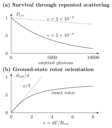
Top: a small per-photon leak accumulates during a long slowing sequence. Bottom: diagonalizing the $m_N=0$ rigid rotor shows how its laboratory dipole departs from $d_{\mathrm{ind}}/d=x/3$, where $x=d\mathcal E/B_{\mathrm{rot}}$. The body-frame dipole is the large-field limit, not the field-free expectation.

Trapping, State Preparation, and Readout

Conservative traps

Static magnetic or electric minima can confine suitable low-field-seeking states. Static fields in a source-free region cannot generally supply a three-dimensional field-magnitude maximum for high-field seekers; dynamic focusing, optical forces, or additional confinement is then needed.

For a nondegenerate internal state $a$, far from absorption, the optical shift uses the peak electric-field amplitude:

$$U_a(\mathbf r)=-\frac14\operatorname{Re} \left[\mathbf E_0^*(\mathbf r)\cdot \boldsymbol{\alpha}_a(\omega_L)\cdot\mathbf E_0(\mathbf r)\right].$$

Near degenerate rotational sublevels, diagonalize the light-shift operator together with Stark, Zeeman, and hyperfine terms. Differential shifts across the occupied wavepacket dephase a superposition even when both states remain trapped. A magic condition for one selected transition need not protect another transition or suppress scattering.

Internal-state preparation

A state label should include every resolved quantum number needed to predict control and collisions. Depending on species and fields, a practical label may be

$$|\alpha;\,v,N,m_N;\,I,m_I;\,\mathcal P\rangle,$$

where $\alpha$ summarizes electronic structure and $\mathcal P$ denotes parity where it remains useful. In intermediate fields, such labels may be only adiabatic correlates; eigenstate composition should then be obtained from a diagonalized effective Hamiltonian.

Microwave, Raman, or adiabatic transfer can select states after cooling. A depletion signal alone confounds state population with transfer and detection efficiency; an independent analysis basis separates these effects.

Readout modalities

Different production routes naturally support different detectors:

• cycling fluorescence: powerful for laser-coolable species, but photon collection and cycling survival must be calibrated;
• reverse association: transfer the molecule back to a Feshbach state, dissociate it, and image the atoms;
• state-selective depletion: remove one internal state and compare surviving populations;
• resonance-enhanced ionization: sensitive and state selective but destructive;
• absorption or fluorescence imaging: useful for ensembles when optical depth and branching are controlled; and
• loss detection in tweezers: site resolved, but intrinsically ambiguous unless molecular loss is distinguished from state transfer.

For a binary molecular-state measurement, write

$$\begin{pmatrix} q_{\mathrm{M}} \\ q_{\mathrm{not\,M}} \end{pmatrix} = \begin{pmatrix} 1-\epsilon_{\mathrm{fn}} & \epsilon_{\mathrm{fp}} \\ \epsilon_{\mathrm{fn}} & 1-\epsilon_{\mathrm{fp}} \end{pmatrix} \begin{pmatrix} p_{\mathrm{M}} \\ p_{\mathrm{not\,M}} \end{pmatrix}.$$

Here $\epsilon_{\mathrm{fn}}$ is the probability that an actual target molecule is reported absent, and $\epsilon_{\mathrm{fp}}$ is the probability that another condition is reported as the target. Inverting this matrix is useful only for a genuine two-class model with known response probabilities and a well-conditioned matrix. Different leaked or lost states need not share the same false-positive probability; one binary measurement cannot resolve arbitrarily many unknown populations.

Electric-Field Control

Rigid-rotor polarization

For a linear rigid rotor with body-frame dipole magnitude $d$,

$$H_{\mathrm{rot+Stark}} = B_{\mathrm{rot}}\frac{\mathbf N^2}{\hbar^2} -d\mathcal E\cos\theta.$$

At zero field, parity makes the laboratory expectation of $d_z$ vanish. For the $N=0$ ground state, the leading coupling is to $N=1,m_N=0$, with matrix element

$$\langle 1,0|\cos\theta|0,0\rangle = \frac{1}{\sqrt3}.$$

When $d\mathcal E\ll B_{\mathrm{rot}}$, second-order perturbation theory gives

$$\Delta E_{00} \approx -\frac{d^2\mathcal E^2}{6B_{\mathrm{rot}}},$$

and the induced dipole is

$$d_{\mathrm{ind}} = -\frac{\partial\Delta E_{00}}{\partial\mathcal E} \approx \frac{d^2\mathcal E}{3B_{\mathrm{rot}}}.$$

This linear low-field result eventually saturates toward the body-frame scale as many rotational states mix. The exact Stark curve should be obtained by diagonalizing enough rotational levels and then checked spectroscopically.

Opposite-parity doublets

Some molecules possess a much smaller opposite-parity splitting $\delta$, expressed here as an energy. Choose state phases so that the dipole matrix element $d_{+-}$ is real. In a two-state model,

$$H_{\mathcal P} = \begin{pmatrix} -\delta/2 & -d_{+-}\mathcal E \\ -d_{+-}\mathcal E & \delta/2 \end{pmatrix}.$$

The lower eigenenergy is

$$E_- = -\sqrt{ \left(\frac{\delta}{2}\right)^2 +d_{+-}^2\mathcal E^2 },$$

so

$$d_{\mathrm{ind}} = -\frac{\partial E_-}{\partial\mathcal E} = \frac{ d_{+-}^2\mathcal E }{ \sqrt{ (\delta/2)^2+d_{+-}^2\mathcal E^2 } }.$$

A small $\delta$ permits strong polarization at modest field. The two-level dipole approaches $|d_{+-}|$, which need not equal the body-frame dipole. Other rotational states must remain sufficiently distant for this truncation. The same strong response makes stray fields consequential.

Dipolar Interactions

Pair interaction

Two laboratory-frame electric dipoles separated by $\mathbf R=R\hat{\mathbf R}$ interact as

$$V_{dd}(\mathbf R) = \frac{1}{4\pi\epsilon_0R^3} \left[ \mathbf d_1\cdot\mathbf d_2 -3 (\mathbf d_1\cdot\hat{\mathbf R}) (\mathbf d_2\cdot\hat{\mathbf R}) \right].$$

For parallel dipoles aligned by a field,

$$V_{dd} = \frac{ d_{\mathrm{ind}}^2 }{ 4\pi\epsilon_0R^3 } \left( 1-3\cos^2\theta \right),$$

where $\theta$ is the angle between the field and the intermolecular axis. The interaction is repulsive side by side, attractive head to tail, and vanishes at the magic angle

$$\cos^2\theta_m = \frac13.$$

This point-dipole form applies when $R$ is large compared with molecular size and the interaction does not strongly mix states omitted from the chosen manifold.

Interaction scale at one micrometre

For

$$d_{\mathrm{ind}} = 1\,\mathrm D = 3.33564\times10^{-30}\,\mathrm{C\,m}$$

and $R=1\,\mu\mathrm m$, the base frequency scale is

$$\begin{aligned} \frac{1}{h} \frac{d_{\mathrm{ind}}^2}{4\pi\epsilon_0R^3} &= 151\,\mathrm{Hz}. \end{aligned}$$

Thus the side-by-side shift is $+151\,\mathrm{Hz}$ and the head-to-tail shift is $-302\,\mathrm{Hz}$. At $R=0.5\,\mu\mathrm m$, the base scale increases by $2^3=8$ to about $1.21\,\mathrm{kHz}$.

The magic-angle zero cancels this leading diagonal point-dipole shift. It does not eliminate higher-order forces or every transition matrix element.

Rotational spin exchange

Choose two rotational states $|\downarrow\rangle$ and $|\uparrow\rangle$. Dipole matrix elements can generate resonant exchange even when each field-free state has zero static dipole. In a pinned array, projection into the two-state manifold often yields

$$H_{\mathrm{spin}} = \sum_{i<j} \left[ \frac{J_{ij}^{\perp}}{2} \left( S_i^+S_j^- +S_i^-S_j^+ \right) +J_{ij}^zS_i^zS_j^z \right] +\sum_i h_iS_i^z.$$

Here $S^z$ has eigenvalues $\pm1/2$, so each $J$ is an energy. For two selected states coupled by a $q=0$ transition dipole $d_t=\langle\uparrow|d_z|\downarrow\rangle$, and diagonal dipoles $d_\uparrow,d_\downarrow$, define

$$A_{ij}=\frac{1-3\cos^2\theta_{ij}}{4\pi\epsilon_0R_{ij}^3}.$$

Keeping resonant exchange but dropping rapidly rotating double excitation gives

$$J_{ij}^{\perp}=2A_{ij}|d_t|^2,\qquad J_{ij}^{z}=A_{ij}(d_\uparrow-d_\downarrow)^2.$$

The mean diagonal dipole also contributes single-spin shifts. Circular ($q=\pm1$) transitions and microwave dressing require their own tensor projection; the same scalar angular factor cannot simply be assumed.

For one resonant pair, starting in $|\uparrow\downarrow\rangle$,

$$P_{\downarrow\uparrow}(t)= \sin^2\!\left(\frac{J^\perp t}{2\hbar}\right).$$

At $t=\pi\hbar/|J^\perp|$, the exchanged amplitude is $-i\,\operatorname{sgn}(J^\perp)$. Positive coupling thus produces the inverse-iSWAP phase in the usual convention, up to local phase corrections. Yan and collaborators observed rotational exchange in pinned molecules.

Collision and loss rates

Define the molecular number-loss coefficient $\beta$ through a homogeneous rate law (including the chosen pair-counting and correlation convention),

$$\frac{dn}{dt} = -\beta n^2,$$

so

$$n(t) = \frac{n_0}{1+\beta n_0t}.$$

The initial two-body loss timescale is

$$\tau_2 = \frac{1}{\beta n_0}.$$

At

$$\beta = 10^{-10}\,\mathrm{cm^3\,s^{-1}}, \qquad n_0 = 10^{11}\,\mathrm{cm^{-3}},$$

one obtains $\tau_2=0.10\,\mathrm s$. Reducing $\beta$ by two orders of magnitude increases this initial timescale to $10\,\mathrm s$, provided one-body loss and heating remain negligible.

For evaporative or rethermalizing collisions, the useful comparison is

$$\gamma_{\mathrm{el/loss}} = \frac{K_{\mathrm{el}}}{K_{\mathrm{loss}}},$$

not the elastic rate alone. Match $K_{\mathrm{loss}}$ to the convention for $\beta$ above; $nK_{\mathrm{el}}$ counts collisions per molecule. A large ratio permits many collisions before loss, but does not directly give the rethermalization rate. Anisotropic dipolar scattering, confinement, and quantum statistics change energy redistribution per collision.

Suppressing short-range encounters

Pinned sites prevent encounters while retaining exchange. In a gas, spin-polarized identical fermions suppress $s$-wave scattering, but remaining partial waves and dipolar attraction can still cause loss. Quasi-two-dimensional confinement with appropriately oriented dipoles can favor repulsive approaches. Microwave shielding instead engineers a repulsive dressed collision channel; its performance depends on polarization, detuning, hyperfine structure, and field geometry (Karman and Hutson).

A longer lifetime at fixed density is useful, but shielding for evaporation also requires sufficient energy redistribution and little added heating. Chemical nonreactivity alone does not exclude complex-mediated loss.

Precision Measurement

Why molecules can be sensitive

Molecular spectra contain ratios of electronic, vibrational, rotational, and hyperfine scales. Some states have strong internal effective electric fields or closely spaced opposite-parity partners. These properties can enhance sensitivity to:

• intrinsic spin-aligned electric dipole moments and other symmetry-violating interactions;
• variation of dimensionless constants;
• nuclear moments and nuclear-spin-dependent effects;
• parity violation; and
• isotope-dependent short-range physics.

The ordinary body-frame dipole of a polar molecule is not itself a time-reversal-violating spin EDM. Enhancement is not accuracy. Closely spaced states are also sensitive to stray fields, geometric phases, leakage, tensor light shifts, and imperfect reversal.

Phase accumulation and sensitivity coefficients

For a Ramsey-like interrogation of duration $T$, a small frequency shift $\delta\omega$ gives

$$\delta\phi = \delta\omega T.$$

For a measured frequency ratio $R=\nu/\nu_{\mathrm{ref}}$ and a dimensionless constant $X$, define

$$K_X^{(R)}=\frac{\partial\ln R}{\partial\ln X},\qquad \frac{\delta R}{R}=K_X^{(R)}\frac{\delta X}{X}.$$

A near-zero splitting can make this fractional coefficient large without increasing the absolute frequency response or the attainable information. Precision molecular measurements develops the comparison and noise limits; cold-molecule frontiers connects these mechanisms to ongoing research.

Exercises

1. Photon-cycle leakage budget

A slowing stage requires $N_\gamma=1.2\times10^4$ scattered photons. Find the largest constant leak probability per photon compatible with (a) 50% and (b) 95% cycle survival. Use the small-leak approximation and check whether it is self-consistent.

Solution

From

$$P_{\mathrm{cyc}} \approx e^{-N_\gamma\epsilon},$$

the leak is

$$\epsilon \approx -\frac{\ln P_{\mathrm{cyc}}}{N_\gamma}.$$

For 50% survival,

$$\begin{aligned} \epsilon_{50} &= \frac{\ln2}{1.2\times10^4} \\ &= 5.78\times10^{-5}. \end{aligned}$$

For 95% survival,

$$\begin{aligned} \epsilon_{95} &= -\frac{\ln0.95}{1.2\times10^4} \\ &= 4.27\times10^{-6}. \end{aligned}$$

Both are much smaller than one, so the exponential approximation is self-consistent. The stricter survival target requires more than an order of magnitude smaller leakage.

2. Recoil and stopping distance

For the $59\,u$, $606\,\mathrm{nm}$ molecule used in the worked example:

1. verify the recoil velocity and photon number needed for $\Delta v=100\,\mathrm{m\,s^{-1}}$;
2. assume an observed scattering rate of $R_{\mathrm{sc}}=2.0\times10^6\,\mathrm{s^{-1}}$ and estimate the slowing time; and
3. estimate the distance traveled under constant deceleration from $100\,\mathrm{m\,s^{-1}}$ to rest.

Solution

The recoil velocity is

$$v_r = \frac{h}{M\lambda} = 1.116\times10^{-2}\,\mathrm{m\,s^{-1}}.$$

Therefore

$$N_\gamma = \frac{100}{1.116\times10^{-2}} = 8.96\times10^3.$$

At the stated scattering rate,

$$t_{\mathrm{slow}} = \frac{N_\gamma}{R_{\mathrm{sc}}} = 4.48\,\mathrm{ms}.$$

Constant deceleration gives mean speed $50\,\mathrm{m\,s^{-1}}$, so

$$L = \frac{v_i+v_f}{2} t_{\mathrm{slow}} = 0.224\,\mathrm m.$$

This idealized result neglects changing Doppler detuning, transverse recoil diffusion, finite laser spectrum, intensity variation, and molecules that leave the cycling manifold.

3. Repump hierarchy

An excited level decays into ground vibrational levels with branching fractions

$$b_0=0.98700, \quad b_1=0.01280, \quad b_2=0.00018, \quad b_{\ge3}=0.00002.$$

Assume every addressed vibrational level is returned perfectly to the same excited level. Estimate the survival after $8000$ photons when the lasers address (a) $v=0,1$ and (b) $v=0,1,2$.

Solution

With $v=0,1$ addressed, the unaddressed probability is

$$\epsilon_{01} = b_2+b_{\ge3} = 2.0\times10^{-4}.$$

Thus

$$P_{01} \approx e^{-8000(2.0\times10^{-4})} = e^{-1.6} = 0.202.$$

With $v=0,1,2$ addressed,

$$\epsilon_{012} = 2.0\times10^{-5},$$

and

$$P_{012} \approx e^{-0.16} = 0.852.$$

One additional repump changes survival by more than a factor of four. The calculation still assumes no rotational, hyperfine, electronic, or off-resonant leakage.

4. Detection before optical pumping into a dark state

Each emitted photon is detected independently with probability $\eta$. After each emission the molecule leaves the optical cycle with probability $\epsilon$, independently of detection; the final emitted photon can be detected. With unlimited illumination, find the mean detected count and the probability of detecting at least one photon before cycling stops.

Solution

The number of emissions is geometric: $P(N=n)=\epsilon(1-\epsilon)^{n-1}$, $n\ge1$. Thus $\langle n_{\mathrm{det}}\rangle=\eta/\epsilon$, whereas

$$P(n_{\mathrm{det}}\ge1) =1-\sum_{n=1}^{\infty}\epsilon(1-\epsilon)^{n-1}(1-\eta)^n =\frac{\eta}{\eta+\epsilon-\eta\epsilon}.$$

For $\eta=0.02,\epsilon=0.001$, the mean is 20 photons but the probability of at least one detection is only 0.953. A large mean does not guarantee negligible false negatives because some molecules leak on an early cycle.

5. Why a round trip can hide failed transfer

In the $\{|f\rangle,|g\rangle\}$ subspace, suppose a coherent forward pulse implements $U=\exp(-i\theta\sigma_y)$ and the reverse pulse implements $U^\dagger$. Starting in $|f\rangle$, compare the target population after one pulse with the return population after both.

Solution

The one-way probability is $\sin^2\theta$, but the roundtrip return probability is one for every $\theta$, including zero. Untransferred amplitude returns coherently too. Inferring one-way efficiency as $\sqrt{P_{\mathrm{return}}}$ requires a population-transfer model with no alternative return pathways, calibrated survival, and equal forward/reverse efficiencies. State-selective removal between passages can test these assumptions; unitarity alone cannot.

6. Polarization and dipolar scale

A linear molecule has body-frame dipole $d=3.0\,\mathrm D$ and rotational constant $B_{\mathrm{rot}}/h=5.0\,\mathrm{GHz}$. In the weak-field $N=0$ limit:

1. find the electric field required for $d_{\mathrm{ind}}=0.30\,\mathrm D$;
2. estimate the side-by-side dipolar interaction frequency for two such induced dipoles separated by $0.75\,\mu\mathrm m$.

Use $d_{\mathrm{ind}}\approx d^2\mathcal E/(3B_{\mathrm{rot}})$.

Solution

The field is

$$\mathcal E = \frac{ 3B_{\mathrm{rot}}d_{\mathrm{ind}} }{ d^2 }.$$

Using

$$B_{\mathrm{rot}} = h(5.0\times10^9\,\mathrm{s^{-1}}),$$

$1\,\mathrm D=3.33564\times10^{-30}\,\mathrm{C\,m}$, and the stated dipoles gives

$$\mathcal E \approx 9.93\times10^4\,\mathrm{V\,m^{-1}} = 0.993\,\mathrm{kV\,cm^{-1}}.$$

The weak-field parameter is

$$\frac{d\mathcal E}{B_{\mathrm{rot}}} \approx 0.30.$$

This is below one but not asymptotically small, so the perturbative value is a useful estimate rather than a precision result. A multilevel Stark diagonalization should replace it for quantitative work.

The interaction frequency scales from the one-Debye, one-micrometre result:

$$\begin{aligned} \frac{V_{dd}}{h} &= (151\,\mathrm{Hz}) \left(\frac{0.30}{1}\right)^2 \left(\frac{1}{0.75}\right)^3 \\ &= 32.2\,\mathrm{Hz}. \end{aligned}$$

This is the side-by-side value. The head-to-tail value would be twice as large in magnitude and negative.

7. Loss and useful collisions

A molecular gas has

$$n_0 = 3.0\times10^{10}\,\mathrm{cm^{-3}}, \quad K_{\mathrm{loss}} = 4.0\times10^{-11}\,\mathrm{cm^3\,s^{-1}},$$

and

$$K_{\mathrm{el}} = 1.2\times10^{-9}\,\mathrm{cm^3\,s^{-1}}.$$

Find the initial two-body loss timescale and the elastic-to-loss ratio. After shielding, $K_{\mathrm{loss}}$ falls by a factor of 20 while $K_{\mathrm{el}}$ falls by a factor of 2. Recompute both quantities and state what else must be measured before claiming improved evaporative cooling.

Solution

Initially,

$$\tau_2 = \frac{1}{K_{\mathrm{loss}}n_0} = \frac{1}{ (4.0\times10^{-11})(3.0\times10^{10}) } = 0.833\,\mathrm s.$$

The rate-coefficient ratio is

$$\gamma_{\mathrm{el/loss}} = \frac{1.2\times10^{-9}}{4.0\times10^{-11}} = 30.$$

After shielding,

$$K_{\mathrm{loss}}' = 2.0\times10^{-12}\,\mathrm{cm^3\,s^{-1}},$$

so

$$\tau_2' = 16.7\,\mathrm s.$$

The elastic coefficient becomes

$$K_{\mathrm{el}}' = 6.0\times10^{-10}\,\mathrm{cm^3\,s^{-1}},$$

and therefore

$$\gamma_{\mathrm{el/loss}}' = 300.$$

The ratio improves by a factor of ten. A cooling claim still requires a measured rethermalization rate, temperature evolution, density and trap calibration, evaporation efficiency, one-body lifetime, and evidence that shielding does not create uncontrolled heating or state mixing.

8. Beyond the weak-field rotor

In the $m_N=0$ basis, use

$$\langle N+1,0|\cos\theta|N,0\rangle =\frac{N+1}{\sqrt{(2N+1)(2N+3)}}$$

to calculate the ground-state energy through fourth order in $x=d\mathcal E/B_{\mathrm{rot}}$. Estimate the correction at $x=0.30$.

Solution

Only $N=0,1,2$ contribute through fourth order. Their diagonal energies in units of $B_{\mathrm{rot}}$ are $0,2,6$, with adjacent couplings $-x/\sqrt3$ and $-2x/\sqrt{15}$. Eliminating the excited components gives

$$e=\frac{x^2/3}{e-2-(4x^2/15)/(e-6)} =-\frac{x^2}{6}+\frac{11x^4}{1080}+O(x^6).$$

Hellmann–Feynman differentiation yields

$$\frac{d_{\mathrm{ind}}}{d}=-\frac{de}{dx} =\frac{x}{3}-\frac{11x^3}{270}+O(x^5).$$

At $x=0.30$, this is $0.0989$ rather than $0.1000$: a 1.1% leading correction. Diagonalizing a larger rotor basis and increasing the cutoff checks the remaining error.

References

• J. L. Bohn, A. M. Rey, and J. Ye, “Cold molecules: Progress in quantum engineering of chemistry and quantum matter,” Science 357, 1002–1010 (2017), doi:10.1126/science.aam6299.
• L. D. Carr, D. DeMille, R. V. Krems, and J. Ye, “Cold and ultracold molecules: science, technology and applications,” New Journal of Physics 11, 055049 (2009), doi:10.1088/1367-2630/11/5/055049.
• N. J. Fitch and M. R. Tarbutt, “Laser cooled molecules,” Advances in Atomic, Molecular, and Optical Physics 70, 157–262 (2021), doi:10.1016/bs.aamop.2021.04.003.
• N. R. Hutzler, “Polyatomic molecules as quantum sensors for fundamental physics,” Quantum Science and Technology 5, 044011 (2020), doi:10.1088/2058-9565/abb9c5.
• N. R. Hutzler, H.-I. Lu, and J. M. Doyle, “The buffer gas beam: An intense, cold, and slow source for atoms and molecules,” Chemical Reviews 112, 4803–4827 (2012), doi:10.1021/cr200362u.
• T. Karman and J. M. Hutson, “Microwave shielding of ultracold polar molecules,” Physical Review Letters 121, 163401 (2018), doi:10.1103/PhysRevLett.121.163401.
• A. Micheli, G. K. Brennen, and P. Zoller, “A toolbox for lattice-spin models with polar molecules,” Nature Physics 2, 341–347 (2006), doi:10.1038/nphys287.
• E. S. Shuman, J. F. Barry, and D. DeMille, “Laser cooling of a diatomic molecule,” Nature 467, 820–823 (2010), doi:10.1038/nature09443.
• B. Yan, S. A. Moses, B. Gadway, J. P. Covey, K. R. A. Hazzard, A. M. Rey, D. S. Jin, and J. Ye, “Observation of dipolar spin-exchange interactions with lattice-confined polar molecules,” Nature 501, 521–525 (2013), doi:10.1038/nature12483.