Bose–Einstein Condensates Overview

A Bose–Einstein condensate is a many-boson state with macroscopic occupation of at least one one-particle natural orbital. In dilute atomic gases, that mode can often be represented by a complex field whose density and phase obey the Gross–Pitaevskii equation. The definition is spectral and many-body; the field equation is an approximation; and an experimental claim is an inference from calibrated observables. Keeping those three levels separate is the central discipline of condensate physics.

The phrase “all atoms occupy the same wavefunction” is useful only as a first idealization. A real gas can contain a thermal component, quantum depletion, several internal states, vortices, fragmented occupations, and finite-size phase fluctuations. A trustworthy analysis therefore reports which mode is macroscopically occupied, which effective theory is being used, and which measurements constrain its assumptions.

Required background. Ultracold atoms introduces degeneracy and interaction scales. Bose–Einstein condensation develops equilibrium state counting; scattering length defines the low-energy coupling used below.

Macroscopic Occupation

The basis-independent definition

For a bosonic field operator $\hat\psi(\mathbf r)$, define the one-body density matrix

$$\rho^{(1)}(\mathbf r,\mathbf r') = \left\langle \hat\psi^\dagger(\mathbf r') \hat\psi(\mathbf r) \right\rangle.$$

It is a positive Hermitian kernel with

$$\int d^3r\, \rho^{(1)}(\mathbf r,\mathbf r) = N.$$

Its spectral decomposition is

$$\rho^{(1)}(\mathbf r,\mathbf r') = \sum_\alpha N_\alpha \phi_\alpha(\mathbf r) \phi_\alpha^*(\mathbf r'),$$

where the orthonormal $\phi_\alpha$ are natural orbitals and the $N_\alpha$ are their occupations. Bose–Einstein condensation occurs when, in the relevant large-system limit,

$$\frac{N_0}{N}\longrightarrow f_0>0.$$

For a simple condensate, one eigenvalue is extensive and the others are subextensive. If several eigenvalues are extensive, the condensate is fragmented. A large occupation in an arbitrarily chosen basis is not the criterion; diagonalizing $\rho^{(1)}$ identifies the physically distinguished modes.

The condensate fraction is

$$f_0 = \frac{N_0}{N}.$$

It is neither the thermal ground-state population in every basis nor the superfluid fraction. The latter is a response coefficient, inferred for example from phase stiffness, nondissipative flow, or rotational response. The two quantities can differ substantially.

Why the trap ground state is not always the condensate orbital

For an equilibrium ideal gas in a static trap with a nondegenerate ground level, the most occupied natural orbital below the transition is the one-particle trap ground state. Interactions deform that orbital. Repulsive interactions broaden it; attraction narrows it and can eventually destabilize the cloud; rotation can produce a vortex texture; multicomponent couplings can produce spinor or fragmented structure.

Thus “ground state” must be qualified:

• one-particle trap ground state refers to the eigenstate of $-\hbar^2\nabla^2/(2m)+V$;
• condensate orbital refers to the leading eigenvector of $\rho^{(1)}$;
• many-body ground state refers to the lowest eigenstate of the full interacting Hamiltonian;
• stationary mean-field state is a critical point of an approximate energy functional.

They coincide only under additional assumptions.

A trapped ideal-gas benchmark

For $N\gg1$ noninteracting bosons in a three-dimensional harmonic trap with geometric-mean angular frequency

$$\bar\omega = \left( \omega_x\omega_y\omega_z \right)^{1/3},$$

the semiclassical transition scale is

$$k_{\mathrm B}T_c^{(0)} = \hbar\bar\omega \left[ \frac{N}{\zeta(3)} \right]^{1/3}.$$

Below this scale, the leading ideal result is

$$\frac{N_0}{N} \simeq 1- \left( \frac{T}{T_c^{(0)}} \right)^3.$$

For $N=10^5$ and $\bar\omega/(2\pi)=100\ \mathrm{Hz}$,

$$T_c^{(0)} \simeq 2.10\times10^{-7}\ \mathrm K = 210\ \mathrm{nK}.$$

This estimate is a scale setter, not a fit formula valid without qualification. Finite-size corrections, interactions, anharmonicity, internal-state mixtures, and imperfect equilibrium all shift the observed crossover. In a finite trap there is no literal thermodynamic singularity; one observes a rapidly growing leading occupation over a finite temperature interval.

From a Mode to an Effective Field

Number-normalized order parameter

When one natural orbital dominates and depletion is modest, define

$$\Psi(\mathbf r,t) = \sqrt{N_0}\, \phi_0(\mathbf r,t) = \sqrt{n_0(\mathbf r,t)} e^{i\theta(\mathbf r,t)}$$

with

$$\int d^3r\, \lvert\Psi(\mathbf r,t)\rvert^2 = N_0.$$

Then $n_0=\lvert\Psi\rvert^2$ is condensate number density. It is not a one-particle probability density. A common alternative normalizes the orbital to one and writes $\Psi=\sqrt{N_0}\phi_0$; mixing these conventions without moving the factor of $N_0$ is a frequent source of wrong nonlinearities.

Writing $\Psi=\sqrt{n_0}e^{i\theta}$ makes the kinematics transparent. The mean-field current and velocity for a scalar field without a vector potential are

$$\begin{aligned} \mathbf j &= \frac{\hbar}{m} \operatorname{Im} \left( \Psi^*\nabla\Psi \right), \\ \mathbf v &= \frac{\mathbf j}{n_0} = \frac{\hbar}{m} \nabla\theta \end{aligned}$$

wherever $n_0\neq0$. Single-valuedness gives quantized circulation around a closed contour that does not cross a node:

$$\oint\mathbf v\cdot d\boldsymbol\ell = \frac{h}{m}\,\ell, \qquad \ell\in\mathbb Z.$$

This connects phase topology to quantized vortices. A prepared phase-winding pattern alone does not measure a superfluid fraction: even a noninteracting wave mode can carry a vortex. Rotational response, vortex stability, and other dynamical information strengthen the interpretation.

The fixed-number caveat

In an exact state with sharp total particle number,

$$\left\langle \hat\psi(\mathbf r) \right\rangle = 0$$

because $\hat\psi$ changes the number sector. The same state can still have an extensive eigenvalue of $\rho^{(1)}$. Therefore $\Psi=\langle\hat\psi\rangle$ is not a universal microscopic definition of condensation.

The complex field can instead be understood as:

• a symmetry-broken representative in the thermodynamic limit;
• a number-conserving condensate orbital multiplied by $\sqrt{N_0}$;
• a relative-phase field defined with respect to another condensate, local oscillator, or measurement record.

A global phase is not observable. Phase differences, currents, interference fringes, and correlation functions are observable.

Gross–Pitaevskii Equation Overview

Contact-interaction model

For one dilute condensate component in three dimensions, with short-range $s$-wave interactions and scattering length $a$, the leading coupling is

$$g = \frac{4\pi\hbar^2a}{m}.$$

The number-normalized Gross–Pitaevskii energy functional is

$$E[\Psi] = \int d^3r\, \bigg[ \frac{\hbar^2}{2m} \lvert\nabla\Psi\rvert^2 + V(\mathbf r) \lvert\Psi\rvert^2 + \frac{g}{2} \lvert\Psi\rvert^4 \bigg].$$

Its closed-system time evolution is

$$i\hbar \frac{\partial\Psi}{\partial t} = \left[ - \frac{\hbar^2\nabla^2}{2m} + V(\mathbf r,t) + g\lvert\Psi\rvert^2 \right] \Psi.$$

For a stationary solution

$$\Psi(\mathbf r,t) = e^{-i\mu t/\hbar} \psi_0(\mathbf r),$$

the equation becomes

$$\mu\psi_0 = \left[ - \frac{\hbar^2\nabla^2}{2m} + V + g\lvert\psi_0\rvert^2 \right] \psi_0.$$

The chemical potential $\mu$ enforces fixed condensate number in the stationary variational problem. It is not generally equal to $E/N_0$ because interaction pairs contribute differently to $E$ and $\mu$.

What the approximation assumes

The equation is reliable when the observable of interest is insensitive to the omitted degrees of freedom. Useful conditions are:

Requirement	Useful diagnostic	Failure sign
three-dimensional dilute gas	$n\lvert a\rvert^3\ll1$	strong quantum depletion or nonuniversal short-range physics
one dominant condensate mode	$N_0/N$ large and unfragmented	several extensive natural occupations
low thermal fraction	thermal density and damping are small	substantial condensate–thermal-cloud exchange
contact interaction	collision energy and range are low	effective-range, dipolar, or multichannel effects
slow coarse-grained dynamics	scales longer than the short-range interaction duration	violent quenches or molecular production
closed conservative evolution	loss and heating times are long	appreciable damping, recombination, or noise

The small gas parameter controls weak-coupling corrections in a stable, repulsive, homogeneous gas. It does not guarantee that every process is slow: three-body recombination, technical noise, or a rapid control ramp can still invalidate a conservative single-field model.

Near a Feshbach resonance, replacing all interaction physics by a very large $g$ is generally unsafe. Unitarity, effective range, loss, molecule formation, and depletion enter before a naive contact mean field becomes arbitrarily strong. Ultracold Atoms gives the corresponding resonance and timescale conditions.

Healing length and sound speed

For a uniform repulsive gas of density $n_0$, the mean-field chemical potential is

$$\mu = gn_0.$$

Balancing kinetic and interaction energies defines the healing length

$$\xi = \frac{\hbar}{\sqrt{2mgn_0}}$$

and long-wavelength density disturbances propagate with sound speed

$$c = \sqrt{\frac{gn_0}{m}}.$$

The two scales obey

$$\xi = \frac{\hbar}{\sqrt{2}\,mc}.$$

The healing length controls how rapidly the field can recover from a hard boundary, density defect, or vortex core. It is not automatically the interparticle spacing or the thermal de Broglie wavelength.

For rubidium-87 with $a=100a_0$ and $n_0=10^{20}\ \mathrm{m^{-3}}$,

$$\begin{aligned} \frac{\mu}{h} &\simeq 773\ \mathrm{Hz}, & \frac{\mu}{k_{\mathrm B}} &\simeq 37.1\ \mathrm{nK}, \\ \xi &\simeq 0.274\ \mu\mathrm m, & c &\simeq 1.88\ \mathrm{mm\,s^{-1}}. \end{aligned}$$

These numbers provide an immediate consistency check. Imaging cannot resolve a bare vortex core if its point-spread function is much broader than $\xi$. For a generic deformation requiring density to redistribute across a cloud of size $R$, the sound-crossing time $R/c$ is a useful adiabaticity scale. It is not a universal speed limit for all controls or specially engineered protocols.

Thomas–Fermi regime

In a repulsive condensate whose interaction energy dominates the kinetic energy over most of the cloud, the stationary density is approximately

$$n_{\mathrm{TF}}(\mathbf r) = \frac{ \mu-V(\mathbf r) }{g} \, \Theta\!\left( \mu-V(\mathbf r) \right).$$

For a harmonic trap

$$V(\mathbf r) = \frac{m}{2} \left( \omega_x^2x^2 + \omega_y^2y^2 + \omega_z^2z^2 \right),$$

the Thomas–Fermi radii satisfy

$$R_i = \sqrt{ \frac{2\mu}{m\omega_i^2} }.$$

The approximation is controlled in the bulk when the cloud dimensions are large compared with the healing length. It necessarily fails in a boundary layer near the sharp Thomas–Fermi edge and at vortex cores, where the kinetic term smooths the density. The complete derivation and normalization formula are derived in the Gross–Pitaevskii equation.

Collective Modes

Uniform excitations

Linearizing about a uniform weakly interacting condensate gives the Bogoliubov dispersion

$$E_k = \sqrt{ \epsilon_k \left( \epsilon_k+2gn_0 \right) }, \qquad \epsilon_k = \frac{\hbar^2k^2}{2m}.$$

At $k\xi\ll1$,

$$E_k \simeq \hbar ck,$$

so the excitation is a collective sound wave. At $k\xi\gg1$,

$$E_k \simeq \epsilon_k+gn_0,$$

and it becomes particle-like. The crossover is physical evidence of interaction-generated rigidity, but extracting it requires a calibrated probe such as Bragg spectroscopy and a model of inhomogeneous broadening.

This dispersion is quoted here for scale interpretation. Its derivation, quasiparticle amplitudes, depletion, zero modes, and stability conditions are developed in Bogoliubov theory.

Modes in a harmonic trap

Confinement discretizes the collective spectrum. In the hydrodynamic Thomas–Fermi limit, low-order modes can often be interpreted as polynomial density and velocity fields:

Mode	Dominant motion	Ideal benchmark in an isotropic trap
dipole	center of mass	$\omega_{\mathrm d}=\omega$
quadrupole surface mode	shape oscillation at nearly fixed volume	$\omega_{\mathrm q}=\sqrt{2}\,\omega$
monopole breathing mode	radial compression and expansion	$\omega_{\mathrm b}=\sqrt{5}\,\omega$

The dipole result is unusually robust. For equal-mass particles with standard quadratic kinetic energy, a common harmonic trap, and interactions depending on relative positions, the total center of mass separates and oscillates at the trap frequency. Internal pair forces cancel in its equation of motion. A shift calls for checking anharmonicity, calibration, spin-dependent traps, synthetic spin–orbit coupling, or whether only one component’s center was measured. Relative motion of two components is not protected by this result.

The quadrupole and breathing frequencies depend on geometry, collisional regime, dimensionality, and equation of state. Their damping can reflect Landau or Beliaev processes, thermal-cloud collisions, dephasing from anharmonicity, or technical noise. A fitted damped sinusoid does not by itself identify the microscopic damping channel.

The hydrodynamic form of the Gross–Pitaevskii equation explains these modes through continuity and force balance. Its quantum-pressure term can be neglected for smooth Thomas–Fermi motion but remains essential near edges and vortex cores. For an experimental comparison, reduce the excitation amplitude to test linear response, and compare an interaction-sensitive mode with the dipole calibration mode using the same trap parameters.

Expansion and Density Profiles

Bimodality

After release, a partly condensed weakly interacting gas often shows a narrow condensate component superposed on a broad thermal distribution. This bimodal structure was central to the first dilute-gas observations. It is persuasive when:

• the thermal wings are fitted in a regime where the assumed distribution is valid;
• the narrow component grows systematically below a reproducible temperature or phase-space-density scale;
• optical depth, saturation, finite resolution, and interactions during expansion are included;
• alternative nonthermal preparation mechanisms are excluded.

A two-component fit is a model comparison, not a direct diagonalization of $\rho^{(1)}$. Report residuals and compare plausible line shapes rather than treating the fit label as the conclusion.

What an absorption image projects

A three-dimensional inverted parabola is not an inverted parabola after line-of-sight integration. For the Thomas–Fermi ellipsoid

$$n(\mathbf r)=n_c\left(1-\frac{x^2}{R_x^2}-\frac{y^2}{R_y^2} -\frac{z^2}{R_z^2}\right)_+,$$

where $(u)_+=\max(u,0)$, integration along $z$ gives

$$n_{\rm col}(x,y)=\frac{4n_cR_z}{3} \left(1-\frac{x^2}{R_x^2}-\frac{y^2}{R_y^2}\right)_+^{3/2}.$$

Integrating the image over $y$ once more gives the line density

$$n_{\rm line}(x)=\frac{\pi n_cR_yR_z}{2} \left(1-\frac{x^2}{R_x^2}\right)_+^2.$$

These quantities have units of inverse volume, area, and length, respectively. Use the correct projection before including imaging resolution or fitting a thermal component.

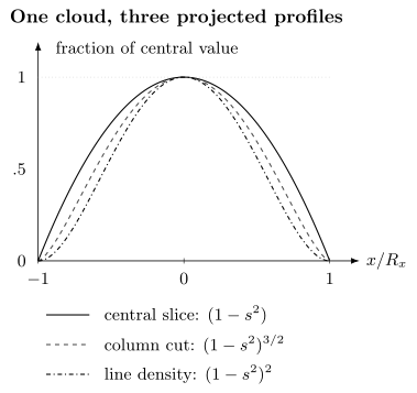
The same ellipsoid gives $(1-s^2)$ for a central three-dimensional slice, $(1-s^2)^{3/2}$ for the central cut through its column image, and $(1-s^2)^2$ for its line density, with $s=x/R_x$. Each curve is divided by its own central value; these are not three clouds with different condensate fractions.

Ballistic and hydrodynamic expansion

For a sufficiently dilute thermal gas, long time of flight approximately maps initial momentum to position,

$$\mathbf r \simeq \frac{\mathbf p}{m}\,t.$$

A condensate can expand nonballistically because mean-field interaction energy is converted into kinetic energy. In the Thomas–Fermi scaling solution, radii evolve as

$$R_i(t) = b_i(t)R_i(0),$$

where, for fixed repulsive $g$ and negligible thermal backaction, after suddenly removing a harmonic trap,

$$\ddot b_i = \frac{\omega_i^2}{ b_i b_xb_yb_z }, \qquad b_i(0)=1, \qquad \dot b_i(0)=0.$$

A tightly confined direction initially has a larger pressure gradient and expands more rapidly. The cloud can therefore invert its aspect ratio. This anisotropic release is a strong consistency check for an interacting condensate, but it is not a unique definition: collisional thermal gases and hydrodynamic Fermi gases can also expand anisotropically.

Interference and Coherence

First-order coherence

The normalized first-order correlation function is

$$g^{(1)}(\mathbf r,\mathbf r') = \frac{ \rho^{(1)}(\mathbf r,\mathbf r') }{ \sqrt{ n(\mathbf r)n(\mathbf r') } }.$$

It measures the visibility available to a one-body interference experiment, after accounting for density. For a perfectly coherent simple condensate in the idealized rank-one limit,

$$\rho^{(1)}(\mathbf r,\mathbf r') = N_0 \phi_0(\mathbf r) \phi_0^*(\mathbf r'),$$

and the condensate contribution factorizes. Thermal occupation, phase fluctuations, multimode structure, and averaging reduce measured coherence.

In an infinite homogeneous three-dimensional condensate, a nonzero large-separation limit of the one-body kernel is one-body off-diagonal long-range order. In finite traps, “long range” is necessarily operational: one compares separations with cloud size, healing length, thermal wavelength, and phase-correlation length. In one and two dimensions, infrared phase fluctuations can replace true long-range order by algebraic or finite-size coherence.

Two expanding condensates

Suppose two initially separated modes overlap after release:

$$\Psi(\mathbf r,t) = \Psi_1(\mathbf r,t) + e^{i\varphi} \Psi_2(\mathbf r,t).$$

The density is

$$n(\mathbf r,t) = \lvert\Psi_1\rvert^2 + \lvert\Psi_2\rvert^2 + 2\operatorname{Re} \left[ e^{i\varphi} \Psi_1^*\Psi_2 \right].$$

For sources separated by $\mathbf d$ and observed after a long expansion time $t$, the far-field fringe wavevector is approximately

$$\mathbf q \simeq \frac{m\mathbf d}{\hbar t},$$

so the fringe spacing along the separation axis is

$$\lambda_{\mathrm{fr}} \simeq \frac{ht}{md}.$$

Independent condensates need not share a reproducible phase before measurement. In a product of two number states, $\langle\hat a_1^\dagger\hat a_2\rangle=0$: the ensemble-mean density has no interference term. Nevertheless, higher-order detection correlations can produce high-contrast fringes in a single many-atom image, with a random phase between repetitions (Javanainen–Yoo). Describing that conditional record with a phase does not establish pre-existing ensemble mutual first-order coherence. Averaging without phase alignment erases the fringes; alignment itself is a data-dependent conditioning step.

What visibility does and does not establish

For local intensities $I_1$ and $I_2$ and mutual degree of coherence $\gamma_{12}$, ideal fringe visibility is

$$\mathcal V = \frac{ 2\sqrt{I_1I_2} }{ I_1+I_2 } \lvert\gamma_{12}\rvert.$$

Low visibility can result from unequal populations, phase noise, imaging resolution, integration along the line of sight, wavefront curvature, or multimode occupation. Conversely, high visibility over one baseline does not reconstruct the full one-body density matrix or prove thermodynamic off-diagonal long-range order. A coherence claim should specify baseline, averaging procedure, phase registration, and transfer function.

Coherent state is a different term

A Glauber coherent state is an eigenstate of an annihilation operator and has number fluctuations. A number-fixed condensate can have a macroscopically occupied natural orbital while not being a Glauber coherent state. “Condensate,” “phase coherent,” and “coherent state” are related but not interchangeable labels.

What Experiments Actually Establish

No single common observable is a complete definition in a finite, interacting, imperfectly measured system. Complementary probes constrain different links in the inference:

Observable	Supports	Important alternatives or nuisance parameters
bimodal density profile	rapidly growing low-momentum component	fit model, resolution, nonequilibrium tails
condensate-fraction trend	occupation transfer below a crossover	thermometry and finite-size corrections
anisotropic expansion	interaction pressure and coherent hydrodynamics	collisional normal-gas hydrodynamics
phase-stable ensemble fringes	mutual first-order coherence on a stated baseline	single-shot fringes can arise without ensemble mutual coherence
collective frequencies	equation of state and mean-field stiffness	anharmonicity and finite temperature
sound propagation	compressibility and hydrodynamic response	damping and inhomogeneous averaging
quantized vortices	phase winding; with dynamics, rotational response	prepared vortices alone do not determine a superfluid fraction
natural-orbital reconstruction	direct occupation spectrum	incomplete tomography and regularization

The most persuasive evidence is overconstrained: one set of calibrated parameters predicts several measurements. For example, atom number, trap frequencies, and scattering length determine a Gross–Pitaevskii density; that density predicts radii, expansion, chemical potential, healing scale, and collective frequencies. Agreement across those observables is harder to mimic than one narrow peak.

Exercises

1. Natural occupations and fragmentation

A sequence of systems has natural occupations

$$N_0=0.70N, \qquad N_1=0.22N, \qquad N_{\alpha\geq2}=O(1).$$

Classify the state in the large-$N$ limit. Would it become a simple condensate if the orbitals were rotated?

Solution

Both $N_0$ and $N_1$ scale linearly with $N$, so the state is a fragmented condensate with at least two macroscopically occupied natural orbitals. A unitary change of one-particle basis changes matrix elements but not the eigenvalues of $\rho^{(1)}$. No basis rotation can combine two extensive eigenvalues into one. A symmetry-breaking perturbation or a change of the many-body state could remove fragmentation, but relabeling the same state cannot.

2. Identical density, different natural occupations

For two orthonormal plane-wave modes of equal local modulus, compare a simple condensate in $(\phi_1+i\phi_2)/\sqrt2$ with an incoherent mixture of equal populations in the two modes. Then randomize the simple condensate’s relative phase between repetitions. Why can an averaged density fail to determine each realization’s occupation spectrum?

Solution

The simple condensate has one-body matrix $N\begin{pmatrix}1&-i\\i&1\end{pmatrix}/2$, with eigenvalues $N,0$. Randomizing its relative phase produces $NI/2$, with eigenvalues $N/2,N/2$. The off-diagonal coherence disappears. The average spatial density is the same as that of the incoherent equal-population state even though each phase-conditioned condensate has a different one-body spectrum. State whether the claimed state is the ensemble or a conditioned realization.

3. Which exponent belongs in the image fit?

Derive the column and line densities above from the three-dimensional Thomas–Fermi ellipsoid. For the normalized central slice, column cut, and line profile, find the half-maximum positions in units of $R_x$.

Solution

Let $A=1-x^2/R_x^2-y^2/R_y^2>0$. Then

$$\int_{-R_z\sqrt A}^{R_z\sqrt A} n_c(A-z^2/R_z^2)\,dz=\frac43 n_cR_z A^{3/2}.$$

Integrating this expression over $y$ uses $\int_{-1}^1(1-u^2)^{3/2}du=3\pi/8$ and yields the line density. For a normalized profile $(1-s^2)^p$, half maximum occurs at $s_{1/2}=\sqrt{1-2^{-1/p}}$. The values for $p=1,3/2,2$ are respectively $0.7071$, $0.6083$, and $0.5412$. Fitting an unprojected parabola to the column image therefore distorts the inferred radius and normalization.

4. Normalization conventions

Let $\phi$ satisfy $\int d^3r\,\lvert\phi\rvert^2=1$ and write $\Psi=\sqrt{N_0}\phi$. Starting from the number-normalized stationary Gross–Pitaevskii equation, derive the equation obeyed by $\phi$.

Solution

Insert $\Psi=\sqrt{N_0}\phi$ into

$$\mu\Psi = \left[ - \frac{\hbar^2\nabla^2}{2m} + V + g\lvert\Psi\rvert^2 \right]\Psi.$$

Since $\lvert\Psi\rvert^2=N_0\lvert\phi\rvert^2$, division by $\sqrt{N_0}$ gives

$$\mu\phi = \left[ - \frac{\hbar^2\nabla^2}{2m} + V + gN_0\lvert\phi\rvert^2 \right]\phi.$$

The factor $N_0$ has not disappeared; it moved into the nonlinear coefficient. Replacing $N_0$ by $N_0-1$ retains exact pair counting in a finite-$N$ Hartree variational state.

5. Thomas–Fermi chemical potential

For an isotropic harmonic trap of angular frequency $\omega$, assume the Thomas–Fermi density

$$n(r) = \frac{\mu-\tfrac12m\omega^2r^2}{g}$$

for $r<R$, and zero outside. Show that

$$N_0 = \frac{8\pi}{15} \frac{\mu R^3}{g}, \qquad R = \sqrt{\frac{2\mu}{m\omega^2}}.$$

Solution

The edge condition $n(R)=0$ gives

$$\mu = \frac12m\omega^2R^2.$$

Normalize the density:

$$\begin{aligned} N_0 &= 4\pi \int_0^R r^2 \frac{ \mu-\tfrac12m\omega^2r^2 }{g} \,dr \\ &= \frac{4\pi}{g} \left[ \frac{\mu R^3}{3} - \frac{m\omega^2R^5}{10} \right]. \end{aligned}$$

Using $m\omega^2R^2=2\mu$,

$$N_0 = \frac{4\pi\mu R^3}{g} \left( \frac13-\frac15 \right) = \frac{8\pi}{15} \frac{\mu R^3}{g}.$$

This derivation also exposes why the density edge is approximate: the neglected kinetic term becomes important where $n$ falls rapidly to zero.

6. Collective-mode consistency

An isotropic trapped condensate has $\omega/(2\pi)=80\ \mathrm{Hz}$. In the Thomas–Fermi hydrodynamic limit, predict the dipole, quadrupole, and monopole frequencies. An experiment instead finds the dipole frequency to be $86\ \mathrm{Hz}$. What should be checked first?

Solution

The ideal frequencies are

$$\begin{aligned} \frac{\omega_{\mathrm d}}{2\pi} &= 80\ \mathrm{Hz}, \\ \frac{\omega_{\mathrm q}}{2\pi} &= \sqrt2 \left( 80\ \mathrm{Hz} \right) \simeq 113\ \mathrm{Hz}, \\ \frac{\omega_{\mathrm b}}{2\pi} &= \sqrt5 \left( 80\ \mathrm{Hz} \right) \simeq 179\ \mathrm{Hz}. \end{aligned}$$

The dipole mode should equal the harmonic-trap frequency independently of translationally invariant interactions. A measured $86\ \mathrm{Hz}$ value therefore calls first for checks of trap calibration, anharmonicity, excitation amplitude, mode identification, component-dependent confinement, and external forces. Ordinary internal pair forces do not shift the total center-of-mass mode under the stated assumptions.

7. Fringe spacing and random phase

Two sodium condensates are separated by $d=40\ \mu\mathrm m$ and overlap after $t=40\ \mathrm{ms}$ of expansion. Estimate their far-field fringe spacing using $m=3.82\times10^{-26}\ \mathrm{kg}$. Explain why averaging many unregistered images can remove the fringes.

Solution

The spacing is

$$\begin{aligned} \lambda_{\mathrm{fr}} &= \frac{ht}{md} \\ &= \frac{ \left( 6.626\times10^{-34}\ \mathrm{J\,s} \right) \left( 4.0\times10^{-2}\ \mathrm s \right) }{ \left( 3.82\times10^{-26}\ \mathrm{kg} \right) \left( 4.0\times10^{-5}\ \mathrm m \right) } \\ &\simeq 1.73\times10^{-5}\ \mathrm m = 17.3\ \mu\mathrm m. \end{aligned}$$

Each realization can acquire a relative phase $\varphi_j$, shifting the fringes. If $\varphi_j$ is uniformly distributed, the ensemble average of $e^{i\varphi_j}$ vanishes. Averaging images before estimating and registering their phases therefore erases the interference term even when individual images have high visibility.

8. Number coherence and pair coherence

Compare a single occupied mode in a number state $|N\rangle$ and in a coherent state with mean $N$. Calculate $\langle\hat a\rangle$, $\langle\hat a^\dagger\hat a\rangle$, and $g^{(2)}=\langle\hat a^{\dagger2}\hat a^2\rangle/N^2$.

Solution

For the number state these quantities are $0$, $N$, and $1-1/N$. For the coherent state they are $\alpha$, $N=|\alpha|^2$, and $1$. Both one-body kernels factorize into the same occupied orbital and have the same mean density. Thus condensation and perfect normalized spatial first-order coherence do not require a nonzero annihilation-operator mean. The number statistics and normally ordered pair correlations still differ.

References

• J. R. Abo-Shaeer, C. Raman, J. M. Vogels, and W. Ketterle, “Observation of Vortex Lattices in Bose–Einstein Condensates,” Science 292, 476–479 (2001), doi:10.1126/science.1060182.
• M. H. Anderson, J. R. Ensher, M. R. Matthews, C. E. Wieman, and E. A. Cornell, “Observation of Bose–Einstein Condensation in a Dilute Atomic Vapor,” Science 269, 198–201 (1995), doi:10.1126/science.269.5221.198.
• M. R. Andrews, C. G. Townsend, H.-J. Miesner, D. S. Durfee, D. M. Kurn, and W. Ketterle, “Observation of Interference Between Two Bose Condensates,” Science 275, 637–641 (1997), doi:10.1126/science.275.5300.637.
• N. N. Bogoliubov, “On the Theory of Superfluidity,” Journal of Physics (USSR) 11, 23–32 (1947), archival scan.
• Y. Castin and R. Dum, “Bose–Einstein Condensates in Time Dependent Traps,” Physical Review Letters 77, 5315–5319 (1996), doi:10.1103/PhysRevLett.77.5315.
• F. Dalfovo, S. Giorgini, L. P. Pitaevskii, and S. Stringari, “Theory of Bose–Einstein Condensation in Trapped Gases,” Reviews of Modern Physics 71, 463–512 (1999), doi:10.1103/RevModPhys.71.463.
• K. B. Davis, M.-O. Mewes, M. R. Andrews, N. J. van Druten, D. S. Durfee, D. M. Kurn, and W. Ketterle, “Bose–Einstein Condensation in a Gas of Sodium Atoms,” Physical Review Letters 75, 3969–3973 (1995), doi:10.1103/PhysRevLett.75.3969.
• E. P. Gross, “Structure of a Quantized Vortex in Boson Systems,” Il Nuovo Cimento 20, 454–477 (1961), doi:10.1007/BF02731494.
• J. Javanainen and S. M. Yoo, “Quantum Phase of a Bose–Einstein Condensate with an Arbitrary Number of Atoms,” Physical Review Letters 76, 161–164 (1996), doi:10.1103/PhysRevLett.76.161.
• D. S. Jin, J. R. Ensher, M. R. Matthews, C. E. Wieman, and E. A. Cornell, “Collective Excitations of a Bose–Einstein Condensate in a Dilute Gas,” Physical Review Letters 77, 420–423 (1996), doi:10.1103/PhysRevLett.77.420.
• A. J. Leggett, “Bose–Einstein Condensation in the Alkali Gases: Some Fundamental Concepts,” Reviews of Modern Physics 73, 307–356 (2001), doi:10.1103/RevModPhys.73.307.
• M. R. Matthews, B. P. Anderson, P. C. Haljan, D. S. Hall, C. E. Wieman, and E. A. Cornell, “Vortices in a Bose–Einstein Condensate,” Physical Review Letters 83, 2498–2501 (1999), doi:10.1103/PhysRevLett.83.2498.
• O. Penrose and L. Onsager, “Bose–Einstein Condensation and Liquid Helium,” Physical Review 104, 576–584 (1956), doi:10.1103/PhysRev.104.576.
• C. J. Pethick and H. Smith, Bose–Einstein Condensation in Dilute Gases, 2nd ed., Cambridge University Press (2008), doi:10.1017/CBO9780511802850.
• L. P. Pitaevskii, “Vortex Lines in an Imperfect Bose Gas,” Soviet Physics JETP 13, 451–454 (1961), archival text.
• L. Pitaevskii and S. Stringari, Bose–Einstein Condensation and Superfluidity, Oxford University Press (2016), doi:10.1093/acprof:oso/9780198758884.001.0001.
• S. Stringari, “Collective Excitations of a Trapped Bose-Condensed Gas,” Physical Review Letters 77, 2360–2363 (1996), doi:10.1103/PhysRevLett.77.2360.