Cavity QED Platforms

A cavity-QED platform places a quantum emitter in a selected resonator mode and engineers both the coherent interaction and the channels through which energy and information leave. The physical platform is not specified by a Jaynes–Cummings Hamiltonian alone. It also contains:

• a resonator geometry and polarization structure;
• an emitter source, trap, or trajectory;
• state preparation and frequency control;
• spatial and angular overlap with the vacuum field;
• useful ports and parasitic loss;
• cavity and emitter stabilization;
• a receiver chain; and
• a calibration model connecting detector records to intracavity dynamics.

The same symbols $g$, $\kappa$, and $\gamma$ can describe a neutral atom between macroscopic mirrors, an ion in a fiber cavity, a Rydberg atom crossing a superconducting microwave resonator, or an emitter near a photonic-crystal defect. The apparatus needed to realize and infer those rates is radically different in each case.

Required background. Cavity QED derives the light–matter response; optical cavities supplies resonator modes; input–output theory supplies port amplitudes; optical dipole traps supplies emitter confinement. Fabricated superconducting emitters are treated in circuit QED.

Cavity Decay and Optical Coherence

Throughout this page,

$$\kappa = \sum_j\kappa_j +\kappa_{\mathrm{int}}$$

is the cavity energy-decay rate. The intracavity photon number decays as $e^{-\kappa t}$, the field amplitude decays as $e^{-\kappa t/2}$, and

$$\frac{\kappa}{2\pi}$$

is the full width at half maximum of an isolated empty-cavity power resonance. The emitter population-decay rate outside the selected cavity channel is $\gamma$, while pure dephasing is $\gamma_\phi$. Its optical coherence rate is

$$\gamma_\perp = \frac{\gamma}{2} +\gamma_\phi.$$

The rate dictionary must be restated when comparing experiments. Some authors call the cavity field-amplitude decay rate $\kappa$, or use $\gamma$ for an atomic half width. Dimensionless numbers agree only after those definitions are translated.

For one designated output port,

$$\eta_{\mathrm{esc}} = \frac{\kappa_{\mathrm{use}}}{\kappa}$$

is the escape fraction conditional on a photon already occupying the cavity mode. It is not the mode-matching efficiency into the cavity, the emitter-to-cavity branching probability, propagation efficiency, or detector efficiency.

From Emitter Preparation to Detected Photons

A useful cavity-QED experiment can be represented as

$$\text{source} \longrightarrow \text{emitter} \longleftrightarrow \text{cavity} \longrightarrow \text{port} \longrightarrow \text{receiver}.$$

Each arrow has its own state space and efficiency. For a generated photon, one possible end-to-end accounting is

$$P_{\mathrm{click}} = P_{\mathrm{prep}} P_{\mathrm{emit}} \beta_{\mathrm{cav}} \eta_{\mathrm{esc}} \eta_{\mathrm{path}} \eta_{\mathrm{det}},$$

where the factors are conditional in sequence:

• $P_{\mathrm{prep}}$ prepares the emitter and motional state;
• $P_{\mathrm{emit}}$ completes the intended control protocol;
• $\beta_{\mathrm{cav}}$ sends the photon into the selected cavity mode;
• $\eta_{\mathrm{esc}}$ sends it through the useful port;
• $\eta_{\mathrm{path}}$ transmits it through filters, fibers, and optics; and
• $\eta_{\mathrm{det}}$ converts the arriving photon into an accepted record.

For these sequential conditional events, the product is the probability chain rule and does not require independence. It fails if one substitutes unconditional efficiencies from different spectral or motional ensembles. For coherent protocols with reabsorption, the event “entered the cavity” need not define an irreversible intermediate step; integrate output flux instead.

Optical Cavity Platforms

Open Fabry–Pérot cavities

Two opposing mirrors form the most direct optical cavity-QED architecture. Its strengths are:

• an open mode volume that can be loaded with neutral atoms, ions, molecules, ensembles, or solid-state samples;
• well-understood Gaussian modes and polarization control;
• independent input and output ports;
• access for trapping, cooling, and control beams; and
• high finesse with low-loss dielectric coatings.

For a weakly dispersive linear cavity of one-way group optical length $L_{\mathrm{opt}}$ (including mirror group delay where relevant),

$$\nu_{\mathrm{FSR}} \approx \frac{c}{2L_{\mathrm{opt}}},$$

and, for an isolated high-finesse resonance,

$$\frac{\kappa}{2\pi} = \delta\nu_{\mathrm{cav}} \approx \frac{\nu_{\mathrm{FSR}}}{\mathcal F}.$$

The approximate standing-wave mode volume

$$V \sim \frac{\pi w_0^2L_{\mathrm{phys}}}{4}$$

shows why short cavities and small waists raise the vacuum field. This estimate assumes a paraxial vacuum standing mode with slowly varying waist; cavity QED explains energy normalization and the limits of a closed-mode volume.

Open access brings engineering costs:

• cavity length noise directly becomes detuning noise;
• mirrors constrain optical access and trap geometry;
• intracavity traps can shift the emitter and cavity coatings can charge;
• transverse modes can approach the working resonance;
• atomic motion samples the standing wave; and
• mirror transmission must be balanced against absorption and scatter.

High finesse is useful only if the cavity can be locked without injecting unacceptable photons, heating, or differential Stark shifts during the quantum sequence.

Fiber Fabry–Pérot cavities

Laser-machined concave structures on fiber facets can produce short cavities with small waists while coupling naturally to fiber modes. They are attractive when compactness and a large $g$ matter.

The small geometry makes the following effects consequential:

• overlap between the cavity eigenmode and the fiber guided mode;
• asymmetric mirror transmissions chosen for a preferred port;
• coating loss and scattering on small curved surfaces;
• birefringence and polarization-mode splitting;
• dielectric charging near trapped ions or atoms;
• limited side access;
• mechanical and thermal stability of the fiber mounts; and
• contamination or damage under vacuum.

The small geometric mode volume is a maximum-coupling statement. Realized performance still depends on placing and cooling the emitter at the correct standing-wave antinode.

Photonic-crystal and nanobeam cavities

Photonic-band-gap defects can confine optical fields to wavelength-scale volumes and route output directly into a waveguide. This can produce a large vacuum field without extreme photon storage time.

Important departures from an open Fabry–Pérot cavity are:

• the emitter samples a strongly varying near field;
• polarization can vary within the mode;
• surfaces are close enough to create Casimir–Polder forces, charging, heating, or spectral shifts;
• fabrication disorder changes resonance frequency, quality factor, and port coupling;
• the cavity may be one-sided only after waveguide and intrinsic losses are separated; and
• quasinormal-mode normalization may be needed in an open or dispersive structure.

For trapped atoms, the nanostructure must be integrated with a stable near-surface trap. For solid-state emitters, implantation position, dipole orientation, spectral diffusion, phonon sidebands, and inhomogeneous fabrication spread replace atomic loading as dominant challenges.

Whispering-gallery and ring resonators

Total internal reflection confines traveling-wave modes around a dielectric boundary. Atoms or other emitters couple to the evanescent field. Advantages include high quality factor, small effective mode volume, and natural waveguide or fiber coupling.

Real devices often support clockwise and counterclockwise modes. Surface roughness couples them and produces standing-wave doublets. An apparent spectral splitting can therefore arise from cavity backscattering before an emitter is introduced. Empty-cavity polarization and direction-mode spectra are essential controls.

Architecture comparison

Optical architecture	Principal strength	Typical dominant constraint	Essential calibration
Macroscopic Fabry–Pérot	Open access and high finesse	Length noise and moderate mode volume	Ringdown, waist, mirror transmissions
Fiber Fabry–Pérot	Small volume and direct fiber interface	Birefringence, access, coating loss	Fiber mode matching and polarization splitting
Photonic crystal	Wavelength-scale volume and integration	Surface physics and fabrication disorder	Local field map and waveguide loss
Whispering-gallery or ring	High $Q$ with evanescent access	Counterpropagating-mode coupling	Empty-cavity doublet and external coupling

No row is uniformly best. The right objective may be coherent swaps, single-pass extinction, high photon extraction, long emitter coherence, parallel fabrication, or optical-network compatibility.

Microwave Cavities with Natural Atoms

Why Rydberg atoms compensate for long wavelength

Microwave modes occupy much larger physical volumes than optical modes, so their zero-point electric field is smaller. Highly excited Rydberg atoms compensate through:

• electric-dipole matrix elements that grow strongly with principal quantum number;
• long radiative lifetimes;
• adjacent transitions in the microwave domain; and
• state-selective field ionization after the atom leaves the cavity.

In traditional microwave cavity QED, circular Rydberg atoms cross a superconducting cavity one by one. Their coupling is time dependent,

$$g(t) = g_0 u[\mathbf r(t)] C_{\mathrm{ang}}(t),$$

and the interaction pulse area is controlled by velocity, trajectory, Stark tuning, and the spatial mode.

The atom is both quantum system and probe. Ramsey zones before and after the cavity can convert a photon-number-dependent phase into an atomic-state probability without absorbing the photon.

Thermal photons

The mean thermal occupation of a mode at angular frequency $\omega_c$ and temperature $T$ is

$$\bar n_{\mathrm{th}} = \frac{1}{ \exp(\hbar\omega_c/k_BT)-1 }.$$

At optical frequency, room-temperature thermal occupation is negligible. At microwave frequency it is an experimental variable.

For

$$\frac{\omega_c}{2\pi} = 51\,\mathrm{GHz},$$

the quantum energy corresponds to

$$\frac{\hbar\omega_c}{k_B} = 2.45\,\mathrm K.$$

Therefore,

$$\bar n_{\mathrm{th}} \approx \begin{cases} 0.049, & T=0.80\,\mathrm K,\\ 1.19, & T=4.0\,\mathrm K,\\ 122, & T=300\,\mathrm K. \end{cases}$$

A cryogenic enclosure, low-emissivity apertures, and thermal filtering are part of state preparation. Measuring the empty-cavity photon statistics is stronger evidence than inferring temperature from a cryostat sensor.

Repeated atom probes

Long photon storage compared with transit time allows several atoms to probe the same field. Off-resonant interactions imprint a photon-number-dependent Ramsey phase while suppressing actual photon exchange. Finite detuning, thermal photons, and atomic velocity spread limit how closely this realizes a nondemolition measurement (Raimond, Brune, and Haroche).

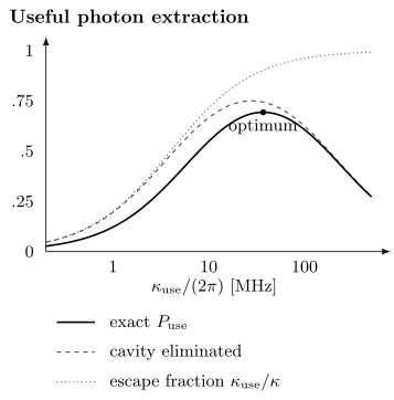
Opening the useful port increases its fraction of cavity loss, but eventually reduces emission into the cavity. The solid curve is the exact probability for a resonant initially excited two-level emitter with no pure dephasing; the dashed curve eliminates the cavity. Rates are $(g,\gamma,\kappa_{\mathrm{loss}})/(2\pi)=(12,3,4)\,\mathrm{MHz}$. The maximum of the solid curve is at $\kappa_{\mathrm{use}}/(2\pi)\simeq37.0\,\mathrm{MHz}$.

Realizing Atom–Cavity Coupling

Maximum versus realized coupling

For a chosen transition, write

$$g(\mathbf r) = g_0 u(\mathbf r) C_{\mathrm{pol}} C_{\mathrm{int}},$$

where:

• $g_0$ is the maximum coupling for a reference dipole at the field maximum;
• $u(\mathbf r)$ is the complex spatial mode normalized to unit maximum;
• $C_{\mathrm{pol}}$ is the projection onto local polarization; and
• $C_{\mathrm{int}}$ contains the angular-momentum matrix element relative to the reference transition.

One useful geometric summary of motion is

$$\langle|g|^2\rangle = g_0^2 \left\langle |u(\mathbf r)|^2 |C_{\mathrm{pol}}|^2 |C_{\mathrm{int}}|^2 \right\rangle.$$

A mean-square coupling does not generally determine a spectrum. For quasistatic motion, average the complex response or detected intensity over the actual distribution; these nonlinear operations do not commute with replacing $|g|^2$ by its mean. Fast motion instead requires a dynamical averaging model.

Standing-wave localization

Near a Fabry–Pérot antinode, a Gaussian standing-wave field may be modeled as

$$u(r,z) = \exp\left(-\frac{r^2}{w_0^2}\right) \cos(kz).$$

For a Gaussian axial position distribution of variance $\sigma_z^2$ centered at $z_0$,

$$\left\langle \cos^2(kz) \right\rangle = \frac12 \left[ 1 + e^{-2k^2\sigma_z^2} \cos(2kz_0) \right].$$

The same mean coupling can arise from a tightly localized atom away from an antinode or a broadly distributed atom centered at one. Sideband spectra, trap-frequency measurements, and position-dependent cavity transmission help distinguish them.

Trapping and cooling inside the mode

Neutral atoms may be delivered by a fountain, conveyor lattice, moving optical tweezer, or loading from a magneto-optical trap. Ions can be held by electrodes while a cavity is positioned around the radio-frequency trap. Flying atomic beams trade long interaction time for simple replenishment.

Intracavity trapping introduces coupled design constraints:

• the trap should localize the emitter where $|g|$ is large;
• differential Stark shifts should not destroy resonance or qubit coherence;
• trap light should not populate or heat the cavity mode;
• cavity cooling or sideband cooling should remove recoil heating;
• the cavity lock should remain stable when control beams switch; and
• a lost emitter should be distinguished from a state change.

Optical tweezers and ion traps explain the corresponding confinement mechanisms.

Multilevel structure

A real alkali atom, ion, molecule, quantum dot, or defect is not exactly a two-level emitter. Cavity polarization and magnetic field select among Zeeman or hyperfine transitions. Off-resonant states can produce:

• additional dispersive shifts;
• Raman scattering and optical pumping;
• polarization rotation;
• dark states;
• leakage outside the qubit manifold; and
• unequal couplings to nominally degenerate cavity polarizations.

An effective two-level model should be checked by varying magnetic field, probe polarization, detuning, and control-state preparation. A fitted $\gamma$ should not silently absorb optical pumping into dark states.

Collective coupling

For $N$ emitters in the weak-excitation limit, the bright collective coupling is

$$G = \sqrt{ \sum_{i=1}^{N} |g_i|^2 }.$$

For equal magnitudes, $G=\sqrt N\,|g|$. This single bright-mode description assumes initially unexcited emitters with sufficiently similar transition frequencies. Inhomogeneous frequencies or linewidths couple bright and dark combinations; one fitted $G$ cannot encode all later dynamics.

Port and Loss Engineering

Useful and parasitic channels

Resolve the total energy decay into physical channels:

$$\kappa = \kappa_1 +\kappa_2 +\kappa_{\mathrm{wg}} +\kappa_{\mathrm{abs}} +\kappa_{\mathrm{sc}} +\cdots.$$

Only selected terms are useful for a given task. A reflection interface may want one dominant input–output port. A transmission experiment needs two ports. A network node may sacrifice storage time to make $\kappa_{\mathrm{use}}/\kappa$ large.

The design trade is explicit:

• decreasing useful transmission can raise finesse and $Q$;
• increasing useful transmission can improve escape and bandwidth;
• intrinsic loss reduces both storage and collection;
• port asymmetry changes the reflected phase and impedance condition.

The loaded linewidth alone cannot separate these contributions. Combine ringdown with calibrated reflection and transmission, or use independent mirror and waveguide characterization.

Mode matching

Let $\eta_{\mathrm{mm}}$ be the incident-power fraction in the selected spatial and polarization mode. In a detector integrating complete orthogonal modes, unmatched prompt reflection adds power without interfering with the cavity mode. A finite aperture or subsequent mode projection can make the detected components overlap and interfere. Spectral mismatch likewise requires the detector’s temporal response.

Thus a power dip is not a direct absorption measurement. Complex reflection, transverse-mode imaging, and a known detection-mode projection distinguish coupling, interference, and loss.

Frequency stabilization

Define detunings

$$\Delta_c = \omega_p-\omega_c, \qquad \Delta_a = \omega_p-\omega_a.$$

Technical fluctuations give distributions of both variables. Cavity length noise, laser noise, magnetic-field noise, ac Stark shifts, and emitter motion can broaden a spectrum in different ways.

An out-of-loop frequency reference can distinguish physical detuning noise from an artificially quiet in-loop error signal. Noise slow compared with a scan produces drift or inhomogeneous broadening; faster noise can dephase the emitter. Neither effect is automatically a Markovian increase of $\gamma$.

Cooperativity as a Platform Metric

Ideal and effective values

With negligible pure dephasing, use

$$C_0 = \frac{4g_0^2}{\kappa\gamma}$$

for maximum single-emitter cooperativity. A motion- and state-averaged value is

$$C_{\mathrm{eff}} = \frac{ 4\langle|g|^2\rangle }{ \kappa\gamma }.$$

If pure dephasing matters, the weak-probe response is instead organized by

$$C_\perp = \frac{ 2\langle|g|^2\rangle }{ \kappa\gamma_\perp }.$$

These are useful averages of local response parameters. For fixed coupling, cooperativity compares cavity and free-space channels; for a broad distribution, $C_{\mathrm{eff}}$ is not generally a sufficient parameter for measured transmission or emission. None of these quantities alone establishes resolved coherent exchange.

Geometry is not the whole metric

For an idealized optical transition and cavity, one often summarizes design as “large $Q/V$.” The realized cooperativity also depends on:

• branching ratio of the selected transition;
• Debye–Waller or zero-phonon fraction for solid-state emitters;
• angular-momentum coefficient;
• position and polarization overlap;
• spectral diffusion and pure dephasing;
• atom number and state purity; and
• additional cavity modes.

Publishing both $C_0$ and $C_{\mathrm{eff}}$, with the reduction factors listed, prevents a simulated field maximum from being mistaken for measured performance.

Worked optical cavity

Consider a linear cavity with

$$\begin{aligned} L &= 200\,\mu\mathrm m, \\ \mathcal F &= 5.00\times10^4, \\ \lambda &= 780\,\mathrm{nm}. \end{aligned}$$

Its free spectral range is

$$\nu_{\mathrm{FSR}} = \frac{c}{2L} = 7.49\times10^{11}\,\mathrm{Hz}.$$

The empty-cavity full width is

$$\frac{\kappa}{2\pi} = \frac{\nu_{\mathrm{FSR}}}{\mathcal F} = 15.0\,\mathrm{MHz}.$$

Thus the energy lifetime is

$$\tau_E = \frac{1}{\kappa} = 10.6\,\mathrm{ns},$$

while the field-amplitude $1/e$ time is $2/\kappa=21.2\,\mathrm{ns}$.

Suppose independent spectroscopy gives

$$\frac{g_0}{2\pi} = 25.0\,\mathrm{MHz}, \qquad \frac{\gamma}{2\pi} = 6.0\,\mathrm{MHz}.$$

Then

$$\begin{aligned} C_0 &= \frac{ 4(25.0)^2 }{ (15.0)(6.0) } \\ &= 27.8. \end{aligned}$$

If motion and internal-state preparation reduce $\sqrt{\langle|g|^2\rangle}$ to $0.70g_0$, then

$$C_{\mathrm{eff}} = (0.70)^2C_0 = 13.6.$$

Both are high-cooperativity values. A strong-coupling claim still requires a comparison of $g$ with the dissipative pole widths and evidence that the observed doublet belongs to one emitter and one cavity mode.

Coherent Exchange and Quantum Signatures

With the energy-decay convention above, the resonant linear amplitude poles are

$$\lambda_\pm=-\frac{\kappa/2+\gamma_\perp}{2} \pm\sqrt{\frac{(\kappa/2-\gamma_\perp)^2}{4}-g^2}.$$

An imaginary part signals underdamped normal modes, but visible peak separation also depends on their width and the measured port. High cooperativity can occur at $\kappa\gg g$, where cavity emission is efficient without several coherent swaps.

An avoided crossing as the emitter is tuned through the cavity, together with empty-cavity mode characterization, identifies coupled emitter–cavity resonances. It does not distinguish a quantized field from classical coupled oscillators in linear response: even oscillatory transients have a classical counterpart (Zhu et al.). Photon antibunching, an excitation-dependent Jaynes–Cummings ladder, or verified emitter–photon entanglement tests additional quantum structure.

Extracting One Prepared Excitation

Prepare $|e,0\rangle$ on resonance with fixed $g$, zero-temperature loss, and $\gamma_\phi=0$. Cavity QED derives the integrated cavity flux,

$$P_{\mathrm{cav}} =\frac{\kappa}{\kappa+\gamma}\frac{C}{1+C}, \qquad C=\frac{4g^2}{\kappa\gamma}.$$

The useful-port probability is therefore

$$P_{\mathrm{use}} =\frac{\kappa_{\mathrm{use}}}{\kappa+\gamma} \frac{4g^2}{4g^2+\kappa\gamma}.$$

The extra $\kappa/(\kappa+\gamma)$ factor accounts for repeated coherent exchange before final decay. The eliminated-cavity result $C/(1+C)$ is recovered for $\kappa\gg g,\gamma$; high cooperativity alone does not justify it. Shaped Raman emission is a different preparation protocol with its own efficiency.

Let $x=\kappa_{\mathrm{use}}$, $\ell=\kappa-\kappa_{\mathrm{use}}$, and $A=4g^2/\gamma$, holding $g,\gamma,\ell$ fixed. Then

$$P_{\mathrm{use}}(x)= \frac{Ax}{(x+\ell+\gamma)(x+\ell+A)}.$$

Differentiation gives the unique positive optimum

$$x_\star=\sqrt{(\ell+\gamma)(\ell+A)}.$$

Opening the port beyond this point reduces the interaction time faster than it improves extraction. In practice, changing mirror transmission may also change geometry or loss; this optimum holds only for the stated fixed parameters.

From a Local Interface to a Quantum Network

A photon source needs both successful extraction and the desired temporal, spectral, and polarization mode. Antibunching constrains multiphoton contamination; it does not establish brightness or indistinguishability. Two-photon interference probes the latter.

For two-photon heralding between nodes, the success probability includes both node-emission probabilities, both channel transmissions, and the interference/detection success. A single-photon heralding protocol has a different loss dependence. State-transfer and gate fidelities must specify whether failed detection, leakage, and lost emitters are retained as erasures or conditioned away. Reiserer and Rempe develop these interface requirements; cavity and circuit QED frontiers discusses extensions to larger systems.

Exercises

1. Linewidth and lifetime conventions

A linear optical cavity has length $L=300\,\mu\mathrm m$ and finesse $\mathcal F=6.0\times10^4$.

1. Find the free spectral range.
2. Find $\kappa/(2\pi)$ under this page’s convention.
3. Find the intracavity energy and field-amplitude $1/e$ times.

Solution

The free spectral range is

$$\nu_{\mathrm{FSR}} = \frac{c}{2L} = 4.997\times10^{11}\,\mathrm{Hz}.$$

The power-resonance full width is

$$\frac{\kappa}{2\pi} = \frac{\nu_{\mathrm{FSR}}}{\mathcal F} = 8.33\,\mathrm{MHz}.$$

Thus

$$\kappa = 2\pi(8.33\times10^6)\,\mathrm{s^{-1}} = 5.23\times10^7\,\mathrm{s^{-1}}.$$

The energy lifetime is

$$\tau_E = \frac{1}{\kappa} = 19.1\,\mathrm{ns}.$$

Since field amplitude decays at $\kappa/2$,

$$\tau_A = \frac{2}{\kappa} = 38.2\,\mathrm{ns}.$$

Calling $1/\kappa$ the amplitude lifetime would create a factor-of-two error.

2. Motion-averaged coupling

An atom is centered at an antinode of

$$u(r,z) = e^{-r^2/w_0^2}\cos(kz).$$

Its axial position is Gaussian with $k\sigma_z=0.30$. Each transverse Cartesian coordinate is Gaussian with $\sigma_r/w_0=0.10$. Internal-state and polarization overlap are ideal. Find $\langle|g|^2\rangle/g_0^2$ and $g_{\mathrm{rms}}/g_0$.

Solution

At an antinode,

$$\left\langle \cos^2(kz) \right\rangle = \frac{ 1+e^{-2k^2\sigma_z^2} }{2} = \frac{1+e^{-0.18}}{2} = 0.918.$$

For two independent transverse Gaussian coordinates,

$$\left\langle e^{-2r^2/w_0^2} \right\rangle = \frac{1}{ 1+4\sigma_r^2/w_0^2 } = \frac{1}{1.04} = 0.962.$$

Therefore

$$\frac{ \langle|g|^2\rangle }{ g_0^2 } = (0.918)(0.962) = 0.883,$$

and

$$\frac{g_{\mathrm{rms}}}{g_0} = \sqrt{0.883} = 0.940.$$

This gives the mean local cooperativity. Averaging an actual transmission spectrum still requires the distribution of $g$, as Exercise 7 demonstrates.

3. High cooperativity without strong coupling

A platform has

$$\frac{g}{2\pi} = 10\,\mathrm{MHz}, \quad \frac{\kappa}{2\pi} = 100\,\mathrm{MHz}, \quad \frac{\gamma}{2\pi} = 0.10\,\mathrm{MHz},$$

with negligible pure dephasing. Find $C$ and classify the regime.

Solution

Common factors of $2\pi$ cancel:

$$C = \frac{4g^2}{\kappa\gamma} = \frac{ 4(10)^2 }{ (100)(0.10) } = 40.$$

The cooperativity is high, so cavity-mediated emission can dominate free-space decay. However,

$$\kappa = 10g,$$

so a cavity excitation leaks much faster than a coherent exchange period. This is a high-cooperativity bad-cavity or Purcell regime, not unambiguous strong coupling.

4. From cavity emission to a click

In the resonant, eliminated-cavity regime $\kappa\gg g,\gamma$, with negligible pure dephasing and one initial emitter excitation, take

$$\beta_{\mathrm{cav}} = \frac{C}{1+C}.$$

For $C=19$, a useful-port fraction $\eta_{\mathrm{esc}}=0.75$, path transmission $\eta_{\mathrm{path}}=0.60$, and detector efficiency $\eta_{\mathrm{det}}=0.80$:

1. find the click probability conditional on successful emitter preparation and emission;
2. compare equal fractional improvements of each efficiency, then equal absolute improvements that remain physically attainable.

Solution

The cavity branching estimate is

$$\beta_{\mathrm{cav}} = \frac{19}{20} = 0.95.$$

The conditional click probability is

$$\begin{aligned} P_{\mathrm{click|emit}} &= (0.95)(0.75)(0.60)(0.80) \\ &= 0.342. \end{aligned}$$

The product gives 34.2%. Equal fractional improvements of any one factor give the same fractional improvement of the product. For equal absolute increments, the smallest factor has the largest logarithmic derivative $\partial\ln P/\partial\eta_i=1/\eta_i$, so path transmission is most effective here. Improving $C$ further has diminishing effect because $C/(1+C)$ is already 0.95. Costs and feasible headroom matter.

The formula assumes matched spectra, independent receiver operation per trial, and the stated cavity elimination.

5. Microwave thermal occupation

For a $51\,\mathrm{GHz}$ cavity:

1. calculate $\hbar\omega_c/k_B$;
2. find $\bar n_{\mathrm{th}}$ at $0.50\,\mathrm K$ and $1.0\,\mathrm K$;
3. find the temperature required for $\bar n_{\mathrm{th}}=0.01$.

Solution

Since $\hbar\omega_c=h\nu_c$,

$$\frac{\hbar\omega_c}{k_B} = \frac{h(51\times10^9)}{k_B} = 2.45\,\mathrm K.$$

At $0.50\,\mathrm K$,

$$\bar n_{\mathrm{th}} = \frac{1}{e^{2.45/0.50}-1} = 7.5\times10^{-3}.$$

At $1.0\,\mathrm K$,

$$\bar n_{\mathrm{th}} = \frac{1}{e^{2.45}-1} = 9.45\times10^{-2}.$$

For a target $\bar n$,

$$\frac{\hbar\omega_c}{k_BT} = \ln\left(1+\frac{1}{\bar n}\right).$$

Thus

$$T = \frac{2.45\,\mathrm K}{\ln101} = 0.530\,\mathrm K.$$

The cavity can still see excess photons from warmer apertures or technical injection even when the local cryostat temperature satisfies this estimate.

6. Port redesign

A cavity has

$$\kappa_{\mathrm{use}} = 2\pi(6\,\mathrm{MHz}), \quad \kappa_{\mathrm{other}} = 2\pi(2\,\mathrm{MHz}), \quad \kappa_{\mathrm{int}} = 2\pi(2\,\mathrm{MHz}).$$

The emitter coupling and decay are

$$\frac{g}{2\pi} = 12\,\mathrm{MHz}, \qquad \frac{\gamma}{2\pi} = 3\,\mathrm{MHz}.$$

Find $\eta_{\mathrm{esc}}$ and $C$. Then double $\kappa_{\mathrm{use}}$ while leaving all other quantities unchanged. Recompute both and explain the trade.

Solution

Initially,

$$\frac{\kappa}{2\pi} = 6+2+2 = 10\,\mathrm{MHz},$$

so

$$\eta_{\mathrm{esc}} = \frac{6}{10} = 0.60.$$

The cooperativity is

$$C = \frac{4(12)^2}{(10)(3)} = 19.2.$$

After doubling the useful coupling,

$$\frac{\kappa'}{2\pi} = 12+2+2 = 16\,\mathrm{MHz},$$

and

$$\eta_{\mathrm{esc}}' = \frac{12}{16} = 0.75.$$

However,

$$C' = \frac{4(12)^2}{(16)(3)} = 12.0.$$

The useful escape fraction improves while storage and cooperativity fall. The best choice depends on whether the protocol is limited by internal channeling, output extraction, bandwidth, or coherent exchange.

7. Why mean coupling can mispredict transmission

For a resonant weak probe in a two-port cavity, normalize transmitted power to its empty-cavity value. With no prompt transmitted path and no pure dephasing, $T(C)=1/(1+C)^2$. Compare an emitter fixed at $C=10$ with a quasistatic ensemble spending equal time at $C=0$ and $C=20$. Both have $\langle C\rangle=10$.

Solution

The fixed emitter transmits $1/121=0.00826$. Averaging detected power for the two configurations gives

$$\langle T\rangle=\frac12\left(1+\frac1{21^2}\right)=0.50113.$$

The large difference comes from the uncoupled half of the sample. A coherent receiver averaging field amplitude would instead average $1/(1+C)$ before forming the selected statistic. Neither measurement is specified by $\langle C\rangle$ alone.

8. Optimal output coupling

For $g/(2\pi)=12\,\mathrm{MHz}$, $\gamma/(2\pi)=3\,\mathrm{MHz}$, and fixed unwanted loss $\ell/(2\pi)=4\,\mathrm{MHz}$, find the useful-port coupling that maximizes the escape probability of one prepared emitter excitation. Does making the port arbitrarily open help?

Solution

In the same frequency units $A/(2\pi)=4(12)^2/3=192\,\mathrm{MHz}$. Therefore

$$\frac{x_\star}{2\pi} =\sqrt{(4+3)(4+192)}\,\mathrm{MHz} =37.0\,\mathrm{MHz}.$$

For $x\to\infty$, $P_{\mathrm{use}}\sim A/x\to0$ even though the cavity escape fraction $x/(x+\ell)$ tends to one. The initially excited emitter then mainly decays outside a cavity that responds too rapidly to build up a field.

References

• A. Boca, R. Miller, K. M. Birnbaum, A. D. Boozer, J. McKeever, and H. J. Kimble, “Observation of the vacuum Rabi spectrum for one trapped atom,” Physical Review Letters 93, 233603 (2004), doi:10.1103/PhysRevLett.93.233603.
• A. D. Boozer, A. Boca, R. Miller, T. E. Northup, and H. J. Kimble, “Reversible state transfer between light and a single trapped atom,” Physical Review Letters 98, 193601 (2007), doi:10.1103/PhysRevLett.98.193601.
• D. Hunger, T. Steinmetz, Y. Colombe, C. Deutsch, T. W. Hänsch, and J. Reichel, “A fiber Fabry–Pérot cavity with high finesse,” New Journal of Physics 12, 065038 (2010), doi:10.1088/1367-2630/12/6/065038.
• H. J. Kimble, “Strong interactions of single atoms and photons in cavity QED,” Physica Scripta T76, 127–137 (1998), doi:10.1238/Physica.Topical.076a00127.
• R. Miller, T. E. Northup, K. M. Birnbaum, A. Boca, A. D. Boozer, and H. J. Kimble, “Trapped atoms in cavity QED: coupling quantized light and matter,” Journal of Physics B 38, S551–S565 (2005), doi:10.1088/0953-4075/38/9/007.
• J.-M. Raimond, M. Brune, and S. Haroche, “Manipulating quantum entanglement with atoms and photons in a cavity,” Reviews of Modern Physics 73, 565–582 (2001), doi:10.1103/RevModPhys.73.565.
• A. Reiserer, “Colloquium: Cavity-enhanced quantum network nodes,” Reviews of Modern Physics 94, 041003 (2022), doi:10.1103/RevModPhys.94.041003.
• A. Reiserer and G. Rempe, “Cavity-based quantum networks with single atoms and optical photons,” Reviews of Modern Physics 87, 1379–1418 (2015), doi:10.1103/RevModPhys.87.1379.
• A. Reiserer, N. Kalb, G. Rempe, and S. Ritter, “A quantum gate between a flying optical photon and a single trapped atom,” Nature 508, 237–240 (2014), doi:10.1038/nature13177.
• H. Ritsch, P. Domokos, F. Brennecke, and T. Esslinger, “Cold atoms in cavity-generated dynamical optical potentials,” Reviews of Modern Physics 85, 553–601 (2013), doi:10.1103/RevModPhys.85.553.
• J. D. Thompson, T. G. Tiecke, N. P. de Leon, J. Feist, A. V. Akimov, M. Gullans, A. S. Zibrov, V. Vuletić, and M. D. Lukin, “Coupling a single trapped atom to a nanoscale optical cavity,” Science 340, 1202–1205 (2013), doi:10.1126/science.1237125.
• H. Walther, B. T. H. Varcoe, B.-G. Englert, and T. Becker, “Cavity quantum electrodynamics,” Reports on Progress in Physics 69, 1325–1382 (2006), doi:10.1088/0034-4885/69/5/R02.
• Y. Zhu, D. J. Gauthier, S. E. Morin, Q. Wu, H. J. Carmichael, and T. W. Mossberg, “Vacuum Rabi splitting as a feature of linear-dispersion theory: Analysis and experimental observations,” Physical Review Letters 64, 2499–2502 (1990), doi:10.1103/PhysRevLett.64.2499.