Quantum Control in AMO

Quantum control is the deliberate steering of a quantum system with time-dependent fields, potentials, measurements, or engineered environments. In atomic, molecular, and optical physics, the programmed controls may be laser amplitudes and phases, microwave voltages, magnetic fields, trap positions, lattice depths, cavity drives, or timed measurements. Their purposes range from a single population transfer to a many-body state preparation, a quantum gate, a spectroscopic interrogation, or stabilization of a nonequilibrium state.

A useful abstract model is

$$H(t;\boldsymbol{\xi}) = H_0(\boldsymbol{\xi}) + \sum_{j=1}^{m} u_j(t)H_j(\boldsymbol{\xi}),$$

where $H_0$ is the drift Hamiltonian, $H_j$ are control operators, $u_j(t)$ are delivered control waveforms, and $\boldsymbol{\xi}$ collects uncertain parameters. The abstraction is powerful, but it hides much of the experimental problem. A waveform stored in an arbitrary-waveform generator is not generally the same waveform seen by an atom. A two-level Hamiltonian may omit neighboring Zeeman states, motional sidebands, spontaneous scattering, field gradients, and correlations between calibration errors.

A successful pulse must accomplish its physical task despite the uncertainties that matter during the experiment. This page compares fixed-axis rotations, adiabatic passage, composite pulses, and constrained optimization.

Required background. Two-level atom supplies the state basis; Rabi oscillations supplies driven rotations; driven open systems supplies time-dependent master equations.

State Transfer and Gate Fidelity

State transfer, gates, and observables

Different tasks require different objective functions. For state transfer from $|\psi_i\rangle$ to $|\psi_{\mathrm{tar}}\rangle$, a natural closed-system fidelity is

$$F_{\mathrm{state}} = \left| \langle\psi_{\mathrm{tar}}| U(T) |\psi_i\rangle \right|^2.$$

This objective says nothing about what $U(T)$ does to states orthogonal to $|\psi_i\rangle$. A gate objective must compare the operation on an entire computational subspace. For a $d$-dimensional closed subspace, one common phase-insensitive unitary overlap is

$$F_{\mathrm{pro}} = \frac{1}{d^2} \left| \operatorname{Tr} \left( U_{\mathrm{tar}}^\dagger U(T) \right) \right|^2.$$

If population can leak out of the subspace, the projected propagator

$$U_P = P U(T)P$$

is not unitary. Reporting only the normalized overlap of $U_P$ can then hide loss. A useful evaluation reports both an in-subspace operation metric and a survival quantity such as

$$S = \frac{1}{d} \operatorname{Tr} \left( U_P^\dagger U_P \right).$$

For coherent evolution in a larger space, count leaked population as failure. Haar averaging over pure inputs in the computational subspace gives

$$F_{\mathrm{avg}} =\frac{\operatorname{Tr}(U_P^\dagger U_P) +|\operatorname{Tr}(U_{\mathrm{tar}}^\dagger U_P)|^2}{d(d+1)} =\frac{S+dF_{\mathrm{pro}}}{d+1},$$

with the unnormalized $F_{\mathrm{pro}}$ computed using $U_P$. For $S=1$ this is the usual unitary average-gate relation; normalizing each surviving output instead answers a different, state-dependent conditional question.

For sensing or spectroscopy, the target may instead be a response. Examples include maximizing a Ramsey fringe slope, minimizing estimator variance, creating a narrow excitation profile, or suppressing response to one frequency band while retaining another. Control quality is always task-relative.

Angular-frequency convention

Unless stated otherwise, $\Omega$, $\Delta$, and $\delta$ denote angular frequencies in radians per second. The corresponding ordinary frequencies are $\Omega/2\pi$, $\Delta/2\pi$, and $\delta/2\pi$ in hertz. For a resonant two-level drive, use $\sigma_z=|e\rangle\langle e|-|g\rangle\langle g|$ and the usual Pauli matrices in the ordered basis $(e,g)$. The rotating-frame Hamiltonian is

$$H_{\mathrm{rot}}(t) = \frac{\hbar}{2} \left[ \Delta(t)\sigma_z + \Omega_x(t)\sigma_x + \Omega_y(t)\sigma_y \right].$$

Define the complex envelope

$$\Omega_c(t) = \Omega_x(t)+i\Omega_y(t) = \Omega(t)e^{i\phi(t)}.$$

With this convention, the control phase $\phi$ sets an equatorial rotation axis

$$\hat{\mathbf n}_\phi = \left( \cos\phi,\, \sin\phi,\, 0 \right).$$

Changing the sign used for $\sigma_y$, the optical phase, or the rotating transformation changes some intermediate formulas. A consistent calibration fixes the physical meaning.

Open-system model

When irreversible processes matter, a commonly used effective model is

$$\dot{\rho} = -\frac{i}{\hbar} \left[ H(t),\rho \right] + \sum_k \mathcal D[L_k]\rho,$$

with

$$\mathcal D[L]\rho = L\rho L^\dagger - \frac{1}{2} \left\{ L^\dagger L,\rho \right\}.$$

The rates and jump operators may themselves depend on the controls. A far-detuned Raman pulse, for example, changes the AC Stark shift and spontaneous-scattering rate when its intensity changes. Treating the dissipator as fixed while optimizing only the coherent Hamiltonian can therefore produce a misleading optimum.

From Programmed Waveform to Physical Control

The control chain

The experimental chain has several layers:

1. a digital representation with a finite sample rate and numerical precision;
2. digital-to-analog conversion, filtering, mixing, amplification, and switching;
3. propagation through cables, fibers, free-space optics, resonators, and impedance mismatches;
4. conversion from field amplitude and polarization to a Hamiltonian matrix element;
5. evolution of the multilevel quantum system; and
6. state preparation and measurement used to infer performance.

A simple linear time-invariant approximation to the first three layers is

$$u_{\mathrm{del}}(t) = \int_{-\infty}^{\infty} h(t-t')u_{\mathrm{prog}}(t')\,dt' + b(t) + n(t),$$

or, in the frequency domain,

$$\widetilde u_{\mathrm{del}}(\omega) = G(\omega) \widetilde u_{\mathrm{prog}}(\omega) + \widetilde b(\omega) + \widetilde n(\omega).$$

A causal response has $h(\tau)=0$ for $\tau<0$. Here $G(\omega)$ is the complex transfer function, $b$ is a systematic offset or drift, and $n$ is stochastic noise. Real chains may also have compression, saturation, hysteresis, frequency conversion, and amplitude-dependent phase. Predistortion based on $G^{-1}$ is useful only over a band where a regularized inverse is stable and the response remains linear. Small $|G|$ amplifies noise; a nonminimum-phase response may not admit a stable causal exact inverse.

The Hamiltonian calibration

Even a perfectly known electric field is not yet a Rabi frequency. For an electric-dipole transition driven by $\mathbf E(t)=\operatorname{Re}[\mathbf E_c e^{-i\omega_dt}]$,

$$\Omega_x-i\Omega_y = -\frac{ \langle e| \mathbf d\mathbin{\cdot}\mathbf E_c |g\rangle }{\hbar}.$$

The matrix element contains angular factors, polarization projections, spatial mode dependence, and possible sums over intermediate states. In a Raman transition, the effective coupling and light shift usually depend differently on intensity and detuning. A calibration should therefore identify the map

$$\left\{ \text{digital controls} \right\} \longrightarrow \left\{ \Omega_x,\Omega_y,\Delta, \text{leakage couplings}, \text{dissipative rates} \right\},$$

not only a single volts-to-hertz conversion.

Identifiability matters

Several parameter changes can produce similar observations. A reduced Rabi contrast may arise from detuning, amplitude inhomogeneity, state-preparation error, readout error, leakage, or decoherence. A single population trace cannot generally distinguish them. Useful calibration experiments vary independent knobs:

• pulse duration and amplitude to reveal coherent frequency;
• drive detuning to produce a chevron;
• phase to identify quadrature signs and imbalance;
• waiting time to separate coherent error from relaxation;
• spatial position or motional state to expose inhomogeneity;
• sequence length to amplify small coherent errors; and
• prepared input state and measurement basis to identify axis errors.

Parameter fitting is not validation when the same data both determine the model and establish its claimed accuracy.

Pulses and Pulse Areas

Resonant rotations

For $\Delta=0$ and constant phase, Hamiltonians at different times commute:

$$\left[ H_{\mathrm{rot}}(t), H_{\mathrm{rot}}(t') \right] = 0.$$

The propagator depends only on the signed pulse area

$$\Theta = \int_{t_i}^{t_f} \Omega(t)\,dt,$$

and is

$$R_\phi(\Theta) = \exp \left[ -\frac{i\Theta}{2} \left( \cos\phi\,\sigma_x + \sin\phi\,\sigma_y \right) \right].$$

A $\pi$ pulse swaps the two basis-state populations up to phases. A $\pi/2$ pulse creates an equal superposition, but the relative phase depends on $\phi$ and on the adopted basis convention. The pulse-area statement fails when detuning, phase, or the rotation axis changes during the pulse, because the Hamiltonians need not commute.

A finite Gaussian pulse

Consider a Gaussian envelope

$$\Omega(t) = \Omega_0 \exp \left[ -\frac{(t-t_0)^2}{2\sigma^2} \right].$$

If the pulse is integrated over a range much wider than $\sigma$,

$$\Theta \simeq \Omega_0\sigma\sqrt{2\pi}.$$

A nominal $\pi$ pulse therefore requires

$$\frac{\Omega_0}{2\pi} = \frac{1}{ 2\sigma\sqrt{2\pi} }.$$

For $\sigma=2.00\ \mu\mathrm{s}$,

$$\frac{\Omega_0}{2\pi} = 99.7\ \mathrm{kHz}.$$

This number is an infinite-support estimate. Truncating the pulse at $t_0\pm 2\sigma$ retains only

$$\operatorname{erf} \left( \frac{2}{\sqrt{2}} \right) \simeq 0.9545$$

of the area. The programmed peak must then be increased by about $4.77\%$ if all other assumptions remain valid. A waveform report that gives $\Omega_0$ and $\sigma$ but not the truncation convention is incomplete.

Detuning and noncommuting errors

For a rectangular pulse with constant $\Omega$, phase zero, and detuning $\Delta$, define

$$\Omega_R = \sqrt{\Omega^2+\Delta^2}.$$

Starting in $|g\rangle$,

$$P_e(t) = \frac{\Omega^2}{\Omega_R^2} \sin^2 \left( \frac{\Omega_Rt}{2} \right).$$

Suppose $\Omega/2\pi=100\ \mathrm{kHz}$ and $\Delta/2\pi=20\ \mathrm{kHz}$. A resonant calibration would choose $t_\pi=5.00\ \mu\mathrm{s}$. At that duration,

$$P_e(t_\pi) = \frac{1}{1+0.2^2} \sin^2 \left[ \frac{\pi}{2} \sqrt{1+0.2^2} \right] \simeq 0.9606.$$

The loss is mainly the tilt of the rotation axis, not a wrong pulse area. Stretching the pulse alone cannot make the maximum transfer exceed

$$P_{e,\max} = \frac{\Omega^2}{\Omega^2+\Delta^2} \simeq 0.9615.$$

Amplitude and phase errors

Let a nominal rotation $R_\phi(\Theta)$ experience a common fractional amplitude error $\epsilon$. The actual angle is

$$\Theta_{\mathrm{act}} = (1+\epsilon)\Theta.$$

For a nominal $\pi$ pulse applied to $|g\rangle$,

$$1-P_e = \sin^2 \left( \frac{\pi\epsilon}{2} \right) = \frac{\pi^2}{4}\epsilon^2 + O(\epsilon^4).$$

A $5\%$ amplitude error therefore gives an idealized transfer error

$$1-P_e \simeq 6.16\times10^{-3}.$$

This quadratic population error should not be confused with the coherent unitary error amplitude, which is first order in $\epsilon$ and can accumulate coherently in a longer sequence.

A constant phase offset rotates the control axis in the equatorial plane. If every pulse and every analysis operation shares the same offset, some measurements are insensitive to it. Relative phase errors between pulses, between sites, or between control and local oscillator are observable and often more consequential.

Spectral selectivity

A pulse of duration $\tau$ necessarily has a finite spectral width. A rectangular envelope produces sinc-like sidelobes, while smooth envelopes reduce abrupt high-frequency content. Selectivity is not determined by duration alone; it depends on the complete complex envelope and on the matrix elements of unwanted transitions.

For a leakage transition detuned by $\Delta_L$, a rough weak-drive scale is

$$P_{\mathrm{leak}} \sim \left| \frac{\Omega_L}{\Delta_L} \right|^2,$$

away from pulse-spectrum zeros and assuming negligible coherent return. Faster control raises $\Omega_L$ and can therefore conflict with state selectivity. Shaping redistributes the error; it does not repeal the bandwidth constraint.

Rotating Frames

Removing the carrier

Consider a laboratory Hamiltonian

$$H_{\mathrm{lab}}(t) = \frac{\hbar\omega_0}{2}\sigma_z + \hbar\Omega_d(t) \cos \left[ \omega_dt+\phi(t) \right] \sigma_x.$$

Choose

$$R(t) = \exp \left( -\frac{i\omega_dt}{2}\sigma_z \right),$$

and define the rotating-frame state

$$|\psi_{\mathrm{rot}}\rangle = R^\dagger(t)|\psi_{\mathrm{lab}}\rangle.$$

The transformed Hamiltonian is

$$H_{\mathrm{rot}} = R^\dagger H_{\mathrm{lab}}R - i\hbar R^\dagger\dot R.$$

After discarding terms oscillating near $2\omega_d$ under the rotating-wave approximation,

$$H_{\mathrm{rot}}(t) \simeq \frac{\hbar}{2} \left[ \Delta\sigma_z + \Omega_d(t) \cos\phi\,\sigma_x + \Omega_d(t) \sin\phi\,\sigma_y \right],$$

where $\Delta=\omega_0-\omega_d$. In particular, a positive laboratory phase in $\cos(\omega_dt+\phi)$ produces the positive-$y$ quadrature here. The upper-right rotating-frame matrix element is $\hbar\Omega_d e^{-i\phi}/2$, which checks both this sign and the complex envelope convention.

The rotating-wave approximation is a model reduction

Dropping the counter-rotating term requires more than a slowly drawn envelope. A representative condition is

$$|\Omega_d|, \ |\Delta|, \ \left|\frac{\dot\Omega_d}{\Omega_d}\right|, \ |\dot\phi| \ll \omega_0+\omega_d,$$

with care near envelope zeros. Strong or ultrafast drives produce counter-rotating effects, including a Bloch–Siegert shift of scale

$$\delta_{\mathrm{BS}} \sim \frac{\Omega_d^2}{4\omega_0}$$

for the near-resonant, weak sinusoidal drive with the amplitude convention specified above. Higher-order terms matter when the drive is strong. In multilevel atoms, additional near-resonant transitions can fail before the two-level counter-rotating term becomes important.

Frequency and phase modulation

If the control phase is time dependent, the instantaneous drive frequency is shifted. Writing the laboratory phase as

$$\Phi_d(t) = \omega_{\mathrm{ref}}t+\phi(t),$$

gives

$$\omega_d(t) = \dot\Phi_d(t) = \omega_{\mathrm{ref}}+\dot\phi(t).$$

Phase ramps and frequency offsets are therefore two descriptions of the same operation. A discontinuity in the digital phase may be a deliberate axis jump, while a discontinuity in phase derivative is a frequency jump. Hardware that resets oscillator phase between pulses can silently change the intended sequence.

A frame dictionary

No single frame is best for every question:

Frame	Transformation removes	Best use	Main caution
Laboratory	nothing	physical frequencies, polarization, hardware phase	carrier obscures slow dynamics
Interaction	selected drift $H_0$	perturbation theory and resonant terms	depends on the chosen partition
Rotating	carrier or local oscillator	pulse axes, detuning, Rabi dynamics	signs and phase conventions vary
Toggling	applied control propagator	error averaging and dynamical decoupling	control imperfections also transform
Dressed	strong static or periodic drive	protected states, Autler–Townes structure	preparation and measurement must be mapped back
Adiabatic	instantaneous eigenbasis	passage and ramps	frame coupling $-i\hbar V^\dagger\dot V$ drives nonadiabatic transitions

For a general unitary frame transformation $V(t)$ with $|\widetilde\psi\rangle=V^\dagger|\psi\rangle$,

$$\widetilde H = V^\dagger HV - i\hbar V^\dagger\dot V.$$

The second term is not optional. It is the source of detuning terms in rotating frames and nonadiabatic couplings in instantaneous eigenbases.

Open systems in a new frame

For a master equation, the jump operators transform too:

$$\widetilde L_k(t) = V^\dagger(t)L_kV(t).$$

A frame change cannot remove physical decoherence. It can make a noise operator time dependent and reveal which spectral components drive transitions between dressed states. Leaving $L_k$ unchanged while transforming only $H$ generally defines a different model.

Adiabatic Passage

Following an instantaneous eigenstate

For the two-level Hamiltonian

$$H(t) = \frac{\hbar}{2} \left[ \Delta(t)\sigma_z + \Omega(t)\sigma_x \right],$$

define

$$\Omega_R(t) = \sqrt{\Delta^2(t)+\Omega^2(t)}$$

and choose a continuous branch of $\theta=\operatorname{atan2}(\Omega,\Delta)$, so that

$$\tan\theta(t) = \frac{\Omega(t)}{\Delta(t)}.$$

The instantaneous eigenstates point parallel and antiparallel to

$$\mathbf h(t) = \left( \Omega(t),0,\Delta(t) \right)$$

on the Bloch sphere. Sweeping $\Delta$ from large negative to large positive values while keeping a nonzero gap can invert the population by following one eigenstate.

In the instantaneous eigenbasis, the geometric coupling has scale

$$\frac{|\dot\theta|}{2},$$

while the eigenfrequency gap is $\Omega_R$. A useful local condition is

$$|\dot\theta| \ll \Omega_R.$$

Equivalently,

$$\left| \Delta\dot\Omega-\Omega\dot\Delta \right| \ll \left( \Delta^2+\Omega^2 \right)^{3/2}.$$

This local ratio is a useful scale test, especially near a small gap. It is not by itself a global error bound: repeated modulation, long accumulation, or abrupt endpoints can still produce transitions. The initial state must match the followed eigenstate, and the whole schedule must be checked.

Linear chirp and the Landau–Zener estimate

For constant $\Omega$ and a linear sweep

$$\Delta(t) = \alpha t$$

extended far beyond the avoided crossing, the ideal Landau–Zener probability of remaining in the same diabatic state (and therefore failing adiabatic inversion) is

$$P_{\mathrm D} = \exp \left( -\frac{\pi\Omega^2}{2|\alpha|} \right).$$

The dimensionless ratio

$$\Lambda = \frac{\Omega^2}{|\alpha|}$$

is therefore a useful first estimate. For a target $P_{\mathrm D}\le 10^{-3}$,

$$\Lambda \ge \frac{2\ln 10^3}{\pi} \simeq 4.40.$$

Finite sweep endpoints, envelope turn-on, decoherence, field inhomogeneity, and extra levels can dominate before this asymptotic formula is accurate.

STIRAP and dark-state passage

STIRAP uses an instantaneous dark state in a three-level system rather than a single avoided crossing. A Stokes pulse precedes and overlaps a pump pulse so that adiabatic following maps the initial state to the target while ideally suppressing occupation of a lossy intermediate state. Its robustness is structured:

• common amplitude variations can preserve the path while changing the adiabatic margin;
• two-photon detuning can directly destroy the dark state;
• finite pulse overlap creates nonadiabatic loss;
• optical phase noise changes transferred coherence; and
• multilevel couplings and differential light shifts modify the nominal three-state Hamiltonian.

The complete derivation and error analysis are at STIRAP.

Robustness, time, and dissipation

Adiabatic passage trades sensitivity to some pulse details for longer exposure and larger integrated control action. If a lossy state has instantaneous occupation $p_\ell(t)$ and decay rate $\Gamma_\ell(t)$, a small-loss estimate is

$$P_{\mathrm{loss}} \simeq \int_0^T \Gamma_\ell(t)p_\ell(t)\,dt.$$

Making a protocol slower can reduce nonadiabatic transitions while increasing this integral. A finite optimum can occur when one error decreases and another increases with duration. It is not automatic: in ideal dark-state passage, slowing can also reduce the lossy-state population, so its integrated exposure need not grow.

Shortcuts to adiabaticity add controls or redesign schedules so that the desired endpoint is reached faster. They are not free: the auxiliary Hamiltonian may require an unavailable operator, greater amplitude, additional bandwidth, or more accurate calibration. A shortcut should be evaluated against the same delivered-control and decoherence constraints as any other pulse.

Composite Pulses

Error cancellation by noncommuting rotations

A composite pulse replaces one intended rotation by a sequence of rotations with chosen phases and angles. Each constituent pulse suffers an error, but the error rotations point along different axes and can cancel order by order.

Write an ideal equatorial rotation as

$$R_\phi(\theta) = \exp \left[ -\frac{i\theta}{2} \sigma_\phi \right],$$

where

$$\sigma_\phi = \cos\phi\,\sigma_x + \sin\phi\,\sigma_y.$$

Under a common fractional pulse-length error $\epsilon$,

$$\widetilde R_\phi(\theta) = R_\phi \left[ (1+\epsilon)\theta \right].$$

The sequence is designed so that its ideal product gives the target and the first several terms in the error expansion vanish.

BB1 for amplitude error

One symmetric BB1 implementation of a target $x$ rotation $R_0(\theta)$, here $0\le\theta\le2\pi$, executes the following pulses in the listed time order:

$$R_0\left(\frac{\theta}{2}\right), \quad R_\phi(\pi), \quad R_{3\phi}(2\pi), \quad R_\phi(\pi), \quad R_0\left(\frac{\theta}{2}\right),$$

with

$$\phi = \arccos \left( -\frac{\theta}{4\pi} \right).$$

For a target $\theta=\pi$,

$$\phi = \arccos \left( -\frac{1}{4} \right) \simeq 104.48^\circ,$$

and $3\phi$ may be reduced modulo $360^\circ$.

In the ideal limit, the middle $\pi$–$2\pi$–$\pi$ correction block is an identity up to global phase. Under a common small amplitude error, its error rotation cancels the leading error of the target pulse. The residual propagator error begins at order $\epsilon^3$, so the small-error infidelity begins at order $\epsilon^6$. A primitive pulse has infidelity of order $\epsilon^2$.

This asymptotic statement is not a universal guarantee. BB1 is much longer than a primitive pulse:

$$\Theta_{\mathrm{tot}} = |\theta|+4\pi.$$

For a $\pi$ target, it accumulates five times the absolute rotation angle. It can therefore suffer more decoherence, off-resonant excitation, time-dependent noise, phase-transient error, and hardware distortion.

Error model determines the sequence

Composite-pulse families target different errors:

Dominant error	Representative strategy	What must be checked
Common pulse-length or amplitude error	BB1, SK1, broadband sequences	phase accuracy, detuning sensitivity, duration
Static detuning or off-resonance error	CORPSE-type sequences	amplitude error, finite bandwidth, sign convention
Simultaneous systematic errors	concatenated or numerically designed sequences	sequence length and cross terms
Spatial selectivity	narrowband or passband sequences	profile over the full spatial distribution
Time-dependent noise	filter-designed control or dynamically corrected gates	noise spectrum and pulse imperfections

A sequence robust to static amplitude error need not reject rapid amplitude noise. The former is an ensemble or calibration uncertainty; the latter is a stochastic process with a spectrum. These require different objective functions.

Static error versus noise during the sequence

The cancellation assumes the same fractional amplitude error on every segment. Independent pulse errors or rapidly changing noise do not share that algebra. Kabytayev et al. examine the noise-frequency dependence of composite control. A scan over amplitude and detuning can distinguish a static amplitude plateau from off-resonance sensitivity.

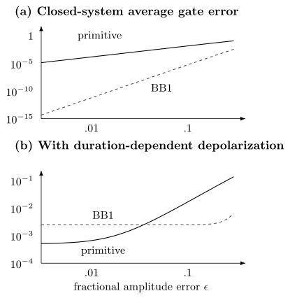
Exact qubit rotations compare a primitive π pulse with symmetric BB1. Top: closed-system average gate infidelity has quadratic versus sixth-order small-error scaling. Bottom: a constant depolarization rate with $\gamma t_\pi=10^{-3}$ adds a larger floor to the five-times-longer BB1 sequence. Near zero amplitude error, the primitive pulse is then better. This illustrative channel is isotropic depolarization, not spontaneous emission.

Optimal Control Overview

Turning a physical task into an objective

Numerical optimal control searches over parameterized waveforms rather than choosing from a small analytic family. A representative objective is

$$J[\mathbf u] = 1-F[\mathbf u] + \lambda_A \sum_j \int_0^T |u_j(t)|^2\,dt + \lambda_S \sum_j \int_0^T |\dot u_j(t)|^2\,dt + \lambda_L L[\mathbf u].$$

The terms can penalize infidelity, control energy, slew or bandwidth, and leakage. Hard constraints may be more appropriate than penalties:

$$|u_j(t)|\le u_{j,\max}, \qquad |\dot u_j(t)|\le s_{j,\max}.$$

Changing the weights changes the question. A pulse described as “optimal” is meaningful only after the objective, constraints, model, duration, and optimization method are stated.

Piecewise-constant propagation

In a common discretization, each control is constant in $N$ intervals of duration $\Delta t$. The propagator is

$$U(T) = U_NU_{N-1}\cdots U_1,$$

with

$$U_n = \exp \left[ -\frac{i\Delta t}{\hbar} \left( H_0+\sum_j u_{j,n}H_j \right) \right].$$

Gradient methods such as GRAPE reuse forward and backward partial propagators to compute derivatives efficiently. Krotov-type methods update controls using forward and adjoint states while enforcing a monotonic improvement property under their assumptions. Basis methods such as CRAB optimize a lower-dimensional waveform expansion. The canonical algorithmic discussion is at Optimal Control.

Robust and ensemble objectives

Let $\boldsymbol{\xi}$ label detuning, intensity scale, position, motional occupation, transfer-function parameters, or other uncertain quantities. An average robust objective is

$$\overline F = \int p(\boldsymbol{\xi}) F(\boldsymbol{\xi})\, d\boldsymbol{\xi},$$

approximated by a weighted sample

$$\overline F \simeq \sum_{r=1}^{N_\xi} w_rF(\boldsymbol{\xi}_r).$$

This is appropriate when $p(\boldsymbol{\xi})$ is a justified operating distribution. A worst-case objective,

$$F_{\min} = \min_{\boldsymbol{\xi}\in\Xi} F(\boldsymbol{\xi}),$$

protects the weakest point in a declared set $\Xi$ but is harder to optimize. A tail-risk objective can interpolate between mean and strict worst case.

Correlations matter. Laser intensity and AC Stark shift may vary together; trap depth, motional frequency, and thermal occupation may not be independent. Sampling each parameter independently can optimize for unphysical combinations while missing the actual uncertainty manifold.

Model-based and closed-loop optimization

A calibrated model can propose a pulse; a few measured correction parameters can compensate static hardware distortion. Optimizing directly against experimental data is also possible (Judson and Rabitz), but the observable must distinguish the intended operation from leakage or a readout artifact. Separate test inputs and parameter values reveal effects that the fitted objective missed.

Controllability is not pulse quality

Lie-algebraic controllability asks whether the available Hamiltonians can generate a desired set of unitaries in an ideal model with sufficient time and admissible controls. It does not answer:

• how long the operation takes;
• how much amplitude or bandwidth it requires;
• whether it is robust;
• whether decoherence destroys it;
• whether the waveform is identifiable from measurements; or
• whether the hardware can deliver it.

Controllability is a reachability statement, not an experimental fidelity claim.

Decoherence, Leakage, and Robustness

Coherent errors can interfere, leakage can return, and state-preparation or measurement bias can imitate a dynamical error. Their “error percentages” are not generally additive. A master equation or an explicit channel composition keeps their effects on the actual observable.

Relaxation during a pulse

Suppose a resonant $\pi$ pulse has duration $t_\pi=5.00\ \mu\mathrm{s}$ and the excited state relaxes with $T_1=1.00\ \mathrm{ms}$. For an ideal resonant rotation from the ground state,

$$p_e(t) = \sin^2 \left( \frac{\pi t}{2t_\pi} \right),$$

whose time average is $1/2$. A first-order jump estimate is

$$P_{\mathrm{jump}} \simeq \int_0^{t_\pi} \frac{p_e(t)}{T_1}\,dt = \frac{t_\pi}{2T_1} = 2.50\times10^{-3}.$$

A jump probability is not the same as final-state infidelity. For this square pulse, first-order amplitude damping gives $1-P_e(t_\pi)=3t_\pi/(8T_1)$, as Exercise 7 derives. A five-times-longer composite sequence may greatly suppress the systematic amplitude error while accumulating a larger relaxation contribution. The crossover must be calculated, not assumed.

Spontaneous scattering in Raman control

For one intermediate state $|i\rangle$ detuned by $\Delta$, write the coupling as

$$H_{\mathrm{int}} =\frac{\hbar}{2}|i\rangle (\Omega_1\langle g|+\Omega_2\langle e|)+\mathrm{h.c.}$$

Adiabatic elimination gives the intermediate amplitude

$$c_i\simeq-\frac{\Omega_1c_g+\Omega_2c_e}{2\Delta}, \qquad \Gamma_{\mathrm{sc}}\simeq\Gamma|c_i|^2.$$

Scattering depends on the evolving lower-state populations and coherence. A dark superposition can cancel this amplitude. The state-independent quantity $\Gamma(|\Omega_1|^2+|\Omega_2|^2)/(4\Delta^2)$ is an upper bound for a normalized lower-state amplitude, not a universal scattering rate. Abrupt switching can add fast transients omitted by this elimination.

The effective Raman coupling scales as $\Omega_1^*\Omega_2/(2\Delta)$. Increasing detuning at fixed optical power slows coherent transfer; keeping that coupling fixed instead requires increasing power. Multilevel interference, differential light shifts, and both forms of scattering must be included in a quantitative optimization.

Leakage and coherent return

Leakage is not always monotonic. An unwanted level may be transiently populated and coherently return by the end of a pulse. Endpoint leakage can therefore be small while transient occupation exposes the system to decay or creates sensitivity to timing. Useful metrics include

$$L_{\mathrm{end}} = 1- \operatorname{Tr} \left[ P\rho(T) \right],$$

and

$$L_{\mathrm{int}} = \int_0^T \left\{ 1- \operatorname{Tr} \left[ P\rho(t) \right] \right\} dt.$$

The first measures final leakage; the second is an exposure measure. Which one matters depends on whether leaked states decay, dephase, collide, or remain detectable.

Quasi-static uncertainty and stochastic noise

An uncertain but constant detuning during one shot should be modeled by an ensemble:

$$\rho(T) = \int p(\Delta) U_\Delta(T)\rho(0)U_\Delta^\dagger(T) \,d\Delta.$$

Rapid detuning noise requires a stochastic or open-system description. Two noise processes with the same variance but different spectra can respond very differently to a pulse sequence. Composite pulses, adiabatic passage, and dynamical decoupling cannot be ranked from a single root-mean-square noise number.

Choosing a Control Strategy

Method-selection map

The following map is a starting point, not a ranking:

Situation	First method to test	Why	Main limitation
Well-isolated transition, accurate resonance, short task	resonant shaped pulse	simple, fast, interpretable	area, detuning, leakage
Dominant repeatable amplitude bias	composite pulse or robust shaped pulse	analytic or numerical cancellation	added duration and phase transients
Broad static detuning distribution	adiabatic rapid passage or robust optimization	follows a gapped eigenstate or trains over ensemble	long exposure and endpoint errors
Lossy intermediate state in a lambda system	STIRAP	dark-state pathway suppresses intermediate occupation	two-photon detuning and phase noise
Dense multilevel spectrum with several constraints	numerical optimal control	uses interference and full model	model mismatch and bandwidth
Slowly drifting hardware	model-assisted closed-loop calibration	updates a small parameter set	estimator bias and overfitting
Time-dependent dephasing noise	filter-designed control or dynamical decoupling	targets a noise spectrum	pulse errors and incompatible signal filtering
State stabilization under ongoing disturbance	measurement feedback or reservoir engineering	continuously removes deviations	latency, inefficiency, backaction

The simplest protocol that meets the task and validation requirements is usually easiest to maintain. Complexity is justified when it removes a measured limitation.

Time-scale hierarchy

Before selecting a method, compare

$$\tau_{\mathrm{carrier}}, \quad \tau_{\mathrm{rise}}, \quad \tau_{\mathrm{ctrl}}, \quad \tau_{\mathrm{noise}}, \quad T_2^*, \quad T_2, \quad T_1, \quad \tau_{\mathrm{drift}}.$$

Here $\tau_{\mathrm{rise}}$ characterizes hardware bandwidth, $\tau_{\mathrm{ctrl}}$ the protocol duration, $\tau_{\mathrm{noise}}$ a relevant noise correlation time, and $\tau_{\mathrm{drift}}$ the calibration lifetime. A typical coherent-control window seeks

$$\tau_{\mathrm{rise}} \ll \tau_{\mathrm{ctrl}} \ll T_1,T_2,$$

but selectivity, adiabaticity, and motional resolution may impose lower bounds on $\tau_{\mathrm{ctrl}}$. There is no universal preference for faster or slower.

Trapped-ion control adds motion and residual spin–motion entanglement; Rydberg blockade adds interaction-dependent leakage; molecular control frontiers explores dense-state and reaction-control problems. These physical constraints determine which of the ideal control constructions remains useful.

Exercises

1. Normalize a truncated Gaussian pulse

A Gaussian Rabi envelope is

$$\Omega(t) = \Omega_0 \exp \left( -\frac{t^2}{2\sigma^2} \right)$$

and is truncated to $|t|\le 2\sigma$.

1. Derive the retained fraction of the infinite-support pulse area.
2. Find $\Omega_0/2\pi$ for a truncated $\pi$ pulse with $\sigma=2.00\ \mu\mathrm{s}$.
3. Explain why matching the area is not sufficient if a constant detuning is present.

Solution

The truncated area is

$$\Theta_{\mathrm{tr}} = \Omega_0 \int_{-2\sigma}^{2\sigma} \exp \left( -\frac{t^2}{2\sigma^2} \right) dt.$$

With $x=t/(\sqrt{2}\sigma)$,

$$\Theta_{\mathrm{tr}} = \Omega_0\sigma\sqrt{2\pi} \operatorname{erf} \left( \sqrt{2} \right).$$

The retained fraction is

$$f_2 = \operatorname{erf} \left( \sqrt{2} \right) \simeq 0.95450.$$

Setting $\Theta_{\mathrm{tr}}=\pi$ gives

$$\frac{\Omega_0}{2\pi} = \frac{1}{ 2\sigma\sqrt{2\pi}f_2 }.$$

For $\sigma=2.00\ \mu\mathrm{s}$,

$$\frac{\Omega_0}{2\pi} \simeq 104.5\ \mathrm{kHz}.$$

With detuning, the rotation axis has a nonzero $z$ component. Hamiltonians with a shaped transverse amplitude and constant detuning generally do not commute at different times, so the final propagator is not determined by the transverse area alone.

2. Compare nominal and detuned pi pulses

A square pulse is calibrated with $\Omega/2\pi=100\ \mathrm{kHz}$ and applied for $t_\pi=5.00\ \mu\mathrm{s}$. During the experiment, $\Delta/2\pi=20.0\ \mathrm{kHz}$.

1. Find the generalized Rabi frequency.
2. Calculate the excited-state probability at $t_\pi$.
3. Find the largest excited-state probability possible without correcting the detuning.
4. Identify a calibration scan that can distinguish detuning from a simple amplitude error.

Solution

The generalized angular frequency is

$$\Omega_R = \sqrt{\Omega^2+\Delta^2},$$

so

$$\frac{\Omega_R}{2\pi} = \sqrt{ (100\ \mathrm{kHz})^2 + (20.0\ \mathrm{kHz})^2 } = 102.0\ \mathrm{kHz}.$$

At the nominal pulse time,

$$P_e = \frac{\Omega^2}{\Omega_R^2} \sin^2 \left( \frac{\Omega_Rt_\pi}{2} \right) = \frac{1}{1.04} \sin^2 \left( \frac{\pi}{2}\sqrt{1.04} \right) \simeq 0.9606.$$

The maximum is the prefactor,

$$P_{e,\max} = \frac{1}{1.04} \simeq 0.9615.$$

A two-dimensional Rabi chevron that scans both drive frequency and pulse duration identifies the resonance center and separates detuning from the on-resonance coupling. A duration scan at only one nominal frequency is more ambiguous.

3. Derive the adiabatic coupling

For

$$H = \frac{\hbar}{2} \left( \Delta\sigma_z+\Omega\sigma_x \right),$$

let

$$\tan\theta = \frac{\Omega}{\Delta}.$$

1. Show that $\dot\theta=(\Delta\dot\Omega-\Omega\dot\Delta)/ (\Delta^2+\Omega^2)$.
2. Compare the geometric coupling to the eigenfrequency gap.
3. For a linear sweep $\Delta=\alpha t$ and constant $\Omega$, state where the local adiabatic condition is hardest to satisfy.

Solution

Differentiate the continuous angle locally (using atan2 through the crossing):

$$\dot\theta = \frac{ \Delta\dot\Omega-\Omega\dot\Delta }{ \Delta^2+\Omega^2 }.$$

A rotation about $y$ diagonalizes the Hamiltonian. Its frame derivative produces an off-diagonal term of magnitude $\hbar|\dot\theta|/2$. The eigenenergy separation is $\hbar\Omega_R$, where

$$\Omega_R = \sqrt{\Delta^2+\Omega^2}.$$

Thus a local adiabatic requirement is

$$|\dot\theta| \ll \Omega_R,$$

or

$$\left| \Delta\dot\Omega-\Omega\dot\Delta \right| \ll \left( \Delta^2+\Omega^2 \right)^{3/2}.$$

For $\Delta=\alpha t$ and constant $\Omega$,

$$|\dot\theta| = \frac{|\alpha|\Omega}{ \alpha^2t^2+\Omega^2 }.$$

The geometric coupling is largest and the gap is smallest at the avoided crossing $t=0$. That is the hardest part of the sweep.

4. Construct a BB1 pi pulse

Use the symmetric BB1 sequence for a target $R_x(\pi)$.

1. Calculate the correction phase $\phi$.
2. List the pulse angles and phases in time order.
3. Find the total absolute rotation angle.
4. Explain why the sequence can perform worse than a primitive pulse even though its static amplitude-error scaling is better.

Solution

For $\theta=\pi$,

$$\phi = \arccos \left( -\frac{\theta}{4\pi} \right) = \arccos \left( -\frac14 \right) \simeq 104.48^\circ.$$

The pulses are, in time order,

$$R_0\left(\frac{\pi}{2}\right), \quad R_\phi(\pi), \quad R_{3\phi}(2\pi), \quad R_\phi(\pi), \quad R_0\left(\frac{\pi}{2}\right).$$

The phase $3\phi\simeq313.43^\circ$ after reduction modulo $360^\circ$. The total absolute angle is

$$\Theta_{\mathrm{tot}} = \frac{\pi}{2}+\pi+2\pi+\pi+\frac{\pi}{2} = 5\pi.$$

BB1 changes the small common amplitude-error infidelity from order $\epsilon^2$ to order $\epsilon^6$, but it is five times as long at fixed Rabi rate. Decoherence, detuning, phase transients, time-dependent noise, and leakage can then outweigh the static-amplitude benefit.

5. Decide when BB1 helps

Compare a primitive $\pi$ pulse with a BB1 $\pi$ pulse. Assume:

• the primitive static amplitude-error contribution is $c_2\epsilon^2$;
• the BB1 contribution is $c_6\epsilon^6$;
• both accumulate an incoherent error at constant rate $\gamma$ per unit absolute rotation angle; and
• BB1 has total angle $5\pi$ while the primitive has angle $\pi$.

1. Write approximate total errors for both.
2. Derive the inequality for BB1 to help.
3. Explain what experimental scan would test the model.

Solution

In this simplified additive model,

$$\varepsilon_{\mathrm{prim}} \simeq c_2\epsilon^2+\gamma\pi,$$

and

$$\varepsilon_{\mathrm{BB1}} \simeq c_6\epsilon^6+5\gamma\pi.$$

BB1 helps when

$$c_2\epsilon^2-c_6\epsilon^6 > 4\gamma\pi.$$

The left side is the coherent-error reduction; the right side is the added incoherent cost. The coefficients depend on the fidelity definition and sequence convention.

Experimentally, impose a calibrated range of amplitude scale errors and measure both protocols, including a duration-matched control and a leakage-sensitive readout. Repeating the sequence several times can amplify coherent residuals. A simultaneous detuning scan checks whether an apparent advantage is confined to one axis.

6. Build a robust-control objective

An optical transition has uncertain fractional intensity scale $s\in[0.9,1.1]$ and detuning $\Delta/2\pi\in[-20,20]\ \mathrm{kHz}$. Population can also leak into $|\ell\rangle$.

1. Propose a sampled average-fidelity objective.
2. Add a final-leakage penalty and a slew penalty.
3. State one reason to prefer a worst-case objective.
4. Give one correlation that independent sampling might miss.

Solution

Choose samples $(s_r,\Delta_r)$ with justified weights $w_r$. One objective to minimize is

$$J = 1- \sum_r w_rF(s_r,\Delta_r) + \lambda_L \sum_r w_r \langle\ell| \rho_r(T) |\ell\rangle + \lambda_S \sum_j \int_0^T |\dot u_j(t)|^2dt.$$

The weights should represent the operating distribution if average performance is the goal. A worst-case objective is useful when every atom, site, or operating point must exceed a threshold and a small bad tail is unacceptable.

Independent sampling could miss a correlation between intensity and AC Stark detuning, because both arise from the same optical field. It could also miss correlations among trap depth, motional frequency, temperature, and coupling.

7. Jump probability versus transfer infidelity

A resonant square π pulse lasts $t_\pi$, with weak spontaneous relaxation $\Gamma=1/T_1$ to $g$. Derive the leading final excited-state error and compare it with the expected number of jumps.

Solution

To first order, insert the ideal trajectory into the dissipator and propagate its contribution through the remaining ideal pulse. At time $t$, let $p=\sin^2(\Omega t/2)$ with $\Omega t_\pi=\pi$. The jump term followed by the remaining rotation contributes $\Gamma p(1-p)$ to final excited population, while the anticommutator contributes $-\Gamma p$. Their sum is $-\Gamma p^2$. Hence

$$1-P_e(t_\pi) =\Gamma\int_0^{t_\pi}\sin^4(\Omega t/2)\,dt+O((\Gamma t_\pi)^2) =\frac{3\Gamma t_\pi}{8}+O((\Gamma t_\pi)^2).$$

The jump count is instead $\Gamma\int p\,dt=\Gamma t_\pi/2$. For $t_\pi=5\,\mu\mathrm s$ and $T_1=1\,\mathrm{ms}$ these are $1.875\times10^{-3}$ and $2.50\times10^{-3}$. A jump need not make the final population completely wrong: the remaining drive can excite the atom again. Gate fidelity involves all input states and is another distinct observable.

8. Perfect surviving output can hide loss

On a two-dimensional computational subspace, let $U_P=\sqrt{s}\,U_{\mathrm{tar}}$, with all missing amplitude transferred to orthogonal leakage states. Find survival, unnormalized process overlap, and average fidelity counting leakage as failure. Then compare a gate $U=\sigma_z$ with target identity on the input $|g\rangle$ alone.

Solution

For state-independent survival, $S=s$, $F_{\mathrm{pro}}=s$, and

$$F_{\mathrm{avg}}=\frac{s+2s}{3}=s.$$

Every normalized surviving output is perfect, but its conditional fidelity one omits probability $1-s$.

For $U=\sigma_z$, the input $|g\rangle$ returns to the same ray, giving state fidelity one. Yet $F_{\mathrm{pro}}=|\operatorname{Tr}\sigma_z|^2/4=0$ and $F_{\mathrm{avg}}=1/3$. An equatorial input reveals the phase error. Successful population transfer alone does not establish a coherent gate.

References

• K. Bergmann, H. Theuer, and B. W. Shore, “Coherent population transfer among quantum states of atoms and molecules,” Reviews of Modern Physics 70, 1003–1025 (1998), doi:10.1103/RevModPhys.70.1003.
• K. R. Brown, A. W. Harrow, and I. L. Chuang, “Arbitrarily accurate composite pulse sequences,” Physical Review A 70, 052318 (2004), doi:10.1103/PhysRevA.70.052318.
• C. Cohen-Tannoudji, J. Dupont-Roc, and G. Grynberg, Atom–Photon Interactions: Basic Processes and Applications (Wiley, 1992).
• H. K. Cummins, G. Llewellyn, and J. A. Jones, “Tackling systematic errors in quantum logic gates with composite rotations,” Physical Review A 67, 042308 (2003), doi:10.1103/PhysRevA.67.042308.
• D. Guéry-Odelin, A. Ruschhaupt, A. Kiely, E. Torrontegui, S. Martínez-Garaot, and J. G. Muga, “Shortcuts to adiabaticity: concepts, methods, and applications,” Reviews of Modern Physics 91, 045001 (2019), doi:10.1103/RevModPhys.91.045001.
• R. S. Judson and H. Rabitz, “Teaching lasers to control molecules,” Physical Review Letters 68, 1500–1503 (1992), doi:10.1103/PhysRevLett.68.1500.
• C. Kabytayev, T. J. Green, K. Khodjasteh, M. J. Biercuk, L. Viola, and K. R. Brown, “Robustness of composite pulses to time-dependent control noise,” Physical Review A 90, 012316 (2014), doi:10.1103/PhysRevA.90.012316.
• N. Khaneja, T. Reiss, C. Kehlet, T. Schulte-Herbrüggen, and S. J. Glaser, “Optimal control of coupled spin dynamics: design of NMR pulse sequences by gradient ascent algorithms,” Journal of Magnetic Resonance 172, 296–305 (2005), doi:10.1016/j.jmr.2004.11.004.
• M. H. Levitt, “Composite pulses,” Progress in Nuclear Magnetic Resonance Spectroscopy 18, 61–122 (1986), doi:10.1016/0079-6565(86)80005-X.
• J. P. Palao and R. Kosloff, “Quantum computing by an optimal control algorithm for unitary transformations,” Physical Review Letters 89, 188301 (2002), doi:10.1103/PhysRevLett.89.188301.
• B. W. Shore, Manipulating Quantum Structures Using Laser Pulses (Cambridge University Press, 2011), doi:10.1017/CBO9780511844222.
• L. M. K. Vandersypen and I. L. Chuang, “NMR techniques for quantum control and computation,” Reviews of Modern Physics 76, 1037–1069 (2005), doi:10.1103/RevModPhys.76.1037.
• N. V. Vitanov, A. A. Rangelov, B. W. Shore, and K. Bergmann, “Stimulated Raman adiabatic passage in physics, chemistry, and beyond,” Reviews of Modern Physics 89, 015006 (2017), doi:10.1103/RevModPhys.89.015006.
• S. Wimperis, “Broadband, narrowband, and passband composite pulses for use in advanced NMR experiments,” Journal of Magnetic Resonance, Series A 109, 221–231 (1994), doi:10.1006/jmra.1994.1159.