Coherent Molecular Control and Its Limits

Molecular control uses fields to change a prepared state, a reaction rate, or a product distribution. Its central resource is the ability to vary quantum amplitudes and their relative phases. Its central difficulty is that a molecule has many coupled degrees of freedom, while an experiment controls and measures only some of them.

This page connects interference, stimulated Raman adiabatic passage, and pulse optimization to observable molecular outcomes. It explains why population transfer, phase preservation, product yield, and selectivity are different achievements. Dated results and open problems are discussed in Molecular control frontiers.

Required background. Quantum control in AMO introduces controllable Hamiltonians; STIRAP develops the three-level dark state; Nonadiabatic coupling explains how electronic and nuclear motion become coupled.

Molecular interference and product probabilities

Suppose a normalized initial superposition can reach a product channel by two routes. Write the product amplitudes as $a$ and $e^{i\phi}b$, including the initial-state coefficients in $a$ and $b$. When the final states are indistinguishable,

$$P_f(\phi)=|a+e^{i\phi}b|^2 =|a|^2+|b|^2+2\operatorname{Re}(a^*b e^{i\phi}).$$

The phase changes the interference term. It does not change the individual pathway strengths. This is the basic coherent-control mechanism discussed by Shapiro and Brumer (2003).

Amplitudes in arbitrary intensity units do not automatically give probabilities. Normalization and the other output channels matter. For example, consider the unitary two-channel map

$$S=\begin{pmatrix}0.8&0.6\\-0.6&0.8\end{pmatrix}, \qquad |\psi_{\rm in}\rangle= \frac{|1\rangle+e^{i\phi}|2\rangle}{\sqrt2}.$$

The probability in output channel 1 is

$$P_1=\frac12+0.48\cos\phi, \qquad P_2=1-P_1.$$

Thus $P_1$ ranges from $0.02$ to $0.98$, always within the probability interval. Destructive interference in one output redistributes probability to the other; it does not destroy normalization. The example represents coherently prepared channels at compatible total energy, or two paths of a driven interferometer with the necessary energy supplied by the fields.

Unobserved motion can reduce interference

If the two paths leave normalized unobserved states $|e_1\rangle$ and $|e_2\rangle$, the part of the final state associated with product $f$ is

$$|f\rangle\otimes \left(a|e_1\rangle+e^{i\phi}b|e_2\rangle\right).$$

Tracing over that unobserved degree of freedom gives

$$P_f=|a|^2+|b|^2+ 2\operatorname{Re}\!\left[ a^*b e^{i\phi}\langle e_1|e_2\rangle\right].$$

An unobserved electron, rotation, or translational wavepacket does not automatically remove interference. Orthogonal final states remove the cross term; partial overlap reduces it. For fixed $a,b$, the visibility is

$$\mathcal V= \frac{2|a b|\,|\langle e_1|e_2\rangle|} {|a|^2+|b|^2}.$$

In a stationary scattering problem, paths must reach compatible outgoing total energies and quantum numbers. Different outgoing kinetic energies can distinguish paths even if only an internal product state is detected. Finite wavepackets require their actual overlap, rather than an assumption that every energy difference is either perfectly resolved or irrelevant.

A thermal mixture is a different issue. If initial states occur incoherently with probabilities $w_j$, then $P_f=\sum_j w_jP_{f|j}$. One adds probabilities across those initial states, while retaining any coherent paths within each $P_{f|j}$. Thermal averaging can wash out a phase dependence when its phase varies across the ensemble.

Dark-state transfer in a molecule

A common molecular preparation problem is to connect a weakly bound state $|1\rangle$ to a deeply bound state $|3\rangle$ through an optically excited state $|2\rangle$. Direct excitation of $|2\rangle$ risks spontaneous decay. STIRAP instead follows a superposition with no excited-state amplitude in the ideal three-level model.

On two-photon resonance, choose real Rabi frequencies and use angular frequencies throughout:

$$\frac{H}{\hbar}=\frac12 \begin{pmatrix} 0&\Omega_P&0\\ \Omega_P&2\Delta&\Omega_S\\ 0&\Omega_S&0 \end{pmatrix}.$$

The dark state is $|D\rangle=\cos\theta|1\rangle-\sin\theta|3\rangle$, with $\tan\theta=\Omega_P/\Omega_S$. Applying the Stokes field first and then changing the pulse ratio moves $\theta$ from $0$ to $\pi/2$. Following $|D\rangle$ then transfers the population to $|3\rangle$. See Vitanov et al. (2017) for the experimental implementations and extensions beyond three levels.

The relevant gap and phase stability

The nonzero eigenfrequencies are

$$\lambda_\pm=\frac{\Delta\pm\sqrt{\Delta^2+\Omega^2}}2, \qquad \Omega=\sqrt{\Omega_P^2+\Omega_S^2}.$$

At one-photon resonance the dark-to-bright gap is $\Omega/2$. At large $|\Delta|$ the smaller gap is approximately $\Omega^2/(4|\Delta|)$. Increasing detuning at fixed laser power therefore makes adiabatic transfer harder. The relevant condition involves the actual coupled eigenstates, $|\langle n|\dot D\rangle|\ll|\lambda_n|$, during the interval in which the state changes.

Relative optical phase also matters. With a phase convention in which

$$|D\rangle=\cos\theta|1\rangle-e^{i\varphi}\sin\theta|3\rangle, \qquad |B\rangle=\sin\theta|1\rangle+e^{i\varphi}\cos\theta|3\rangle,$$

direct differentiation gives

$$|\langle B|\dot D\rangle|^2 =\dot\theta^2+\sin^2\theta\cos^2\theta\,\dot\varphi^2.$$

The phase term is largest near equal pump and Stokes strengths. A criterion using only $|\dot\theta|$ misses it. In a rotating frame that absorbs a time-dependent phase into a basis state, the same physics appears as an additional detuning. These are two descriptions of one effect.

Longer pulses can reduce changes in the mixing angle while allowing more dephasing, loss, and drift. Real molecules also have nearby excited levels, polarization-dependent couplings, and spatially varying light shifts. Consequently, the useful duration is determined by both adiabaticity and the available coherence time, rather than by pulse length alone.

Repeated transfer and phase preservation

If each transfer retains a fraction $\eta$ in the intended state and all failures are irreversible and independent, then $N$ transfers retain

$$S_N=\eta^N.$$

A round trip contains two transfers. Under identical forward and reverse efficiencies, $n$ round trips give $S_{2n}=\eta^{2n}$. Unequal directions instead give $(\eta_{\rightarrow}\eta_{\leftarrow})^n$. A survival curve alone determines their product, not the two efficiencies separately.

This simple model can fail in instructive ways. Coherently leaked amplitude can return on a later pulse. Molecules at different positions can also have different but persistent transfer efficiencies. If half the molecules have $\eta=0.99$ and half have $\eta=0.90$, with independent irreversible failures within each group, then

$$S_N=\frac12(0.99^N+0.90^N),$$

which is not $0.945^N$. The remaining ensemble becomes enriched in the better-transferred group. Fitting a single per-transfer efficiency without allowing for this heterogeneity can obscure the underlying distribution.

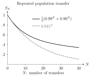
Both ensembles retain $94.5\%$ after one transfer. Their later survival differs because a molecule’s transfer efficiency remains correlated across cycles in the two-group model. The curves describe population retention, not a phase-sensitive gate test.

Even perfect population transfer of one input does not imply a coherent gate on arbitrary superpositions. For example, a channel can map each basis state to the desired basis state while erasing the relative phase between them. A Ramsey interference measurement probes that missing coherence; a complete gate assessment also includes other inputs and leakage. The distinction is developed in Quantum control in AMO and AMO platforms.

Pulse shaping with a physical objective

In an idealized dipole model, a field changes the Hamiltonian through $H(t)=H_0-\mathbf d\cdot\mathbf E(t)$. For a target subspace with projector $\Pi$, the quantity

$$F_\Pi=\operatorname{Tr}[\Pi\rho(T)]$$

is its final population. It equals overlap with a specified pure target state when $\Pi$ has rank one. For a larger subspace, it does not specify which state or coherence has been prepared inside that subspace.

The field at the molecule may differ from the commanded waveform. A linear response model is

$$E_{\rm sample}(t)=\int h(t-t')u(t')\,dt',$$

with $u$ the command and $h$ the measured response. A calculated pulse may contain features that a modulator, amplifier, or optical path cannot deliver. Including the response in forward propagation avoids assuming that an unstable inverse filter can reconstruct every desired field. Rasulov and Kuprov (2025) discuss this approach in optimal control.

A possible optimization objective is

$$J=\mathbb E_\xi[F_\Pi(u,\xi)] -\lambda\operatorname{Var}_\xi[F_\Pi(u,\xi)] -\alpha\int |u(t)|^2dt,$$

where $\xi$ describes uncertain detunings, intensities, or molecular parameters. The coefficients must give the terms consistent units. The variance penalty discourages sensitivity over the chosen distribution; it does not guarantee good performance at every parameter value. A worst-case target requires an explicitly worst-case objective or constraints.

Similarly, a penalty on $\int|\dot u|^2dt$ favors smooth pulses but does not enforce a strict bandwidth limit. Hard amplitude, bandwidth, and duration limits should be imposed as constraints or built into the pulse basis. General control methods are developed in Optimal control; Koch et al. (2022) review their wider use.

Product yield, selectivity, and the detector

Let $Y_f$ be the number of target products per fixed incident exposure, and let $Y_{\rm all}$ be the corresponding total number of reaction products. The branching fraction is $B_f=Y_f/Y_{\rm all}$. A pulse can increase $Y_f$ while decreasing $B_f$ by increasing unwanted products still more strongly. Both can be useful objectives, but they answer different questions.

Detected counts need not be proportional to all products with the same constant. Ionization probability, collection angle, and detector efficiency may depend on the product state. Changing the pulse can also alter these readout processes. To infer molecular selectivity from a count ratio, one needs a model or calibration connecting each count channel to its products.

Feedback optimization can find a better pulse even when the molecular model is incomplete. The resulting signal improvement does not uniquely identify the mechanism. Varying a physically motivated parameter, such as phase, polarization, delay, or detuning, and predicting the resulting trend makes the mechanism more specific than the optimized signal alone.

Coupled electronic and nuclear motion

Near nonadiabatic regions, a pulse changes a wavepacket moving on coupled electronic potential surfaces. It may alter where the packet reaches a crossing, its momentum distribution, or the relative phase between components. A final product ratio compresses this time-dependent motion into one number, so different trajectories can produce the same ratio.

When comparing calculations, specify the observable. A population assigned to a chosen diabatic basis and a projection onto an adiabatic electronic eigenspace need not agree: they describe different decompositions. For a nondegenerate adiabatic state, the projector is unchanged by an arbitrary phase choice. Within an exactly degenerate eigenspace, its total projector is well defined while individual basis-state populations depend on the chosen basis. Physical predictions must be transformed consistently.

Conical intersections and Nonadiabatic coupling develop these issues. For experimental interpretation, combine product distributions with time-dependent observables that a candidate dynamical model also predicts. This narrows the possible mechanisms without assuming that one fitted population curve determines the full molecular wavefunction.

Common pitfalls

Alignment and orientation are different. For a molecular axis making angle $\vartheta$ with a laboratory direction, $\langle\cos^2\vartheta\rangle$ measures alignment and $\langle\cos\vartheta\rangle$ measures head-to-tail orientation. An isotropic ensemble has values $1/3$ and $0$, respectively; a strongly aligned ensemble can still have zero orientation.

Conditioning changes the question. Fidelity among retained molecules does not include lost molecules. Give the retention probability alongside a conditional state quality so that the whole preparation process is clear.

Population transfer is input specific. A good result for one initial state is a state-preparation result. A claim about a gate requires its action on a suitable set of inputs, including superpositions.

Exercises

Interference with normalized channels

For the two-channel matrix above, find the largest and smallest $P_1$, its visibility, and the incoherent-mixture result. Why can the probability not exceed one?

Solution

The extrema are $0.98$ and $0.02$, so $\mathcal V=(0.98-0.02)/(0.98+0.02)=0.96$. For the equal incoherent mixture, $P_1=(0.8^2+0.6^2)/2=0.5$. The initial vector is normalized and $S^\dagger S=I$, so the output probabilities sum to one. Using arbitrary unnormalized pathway strengths would not provide this guarantee.

A dark-state gap and a changing phase

Take $\Omega=2\pi\times1\ {\rm MHz}$ and $\Delta=2\pi\times10\ {\rm MHz}$. Find the smaller dark-to-bright gap in hertz. At $\theta=\pi/4$, $\dot\theta=0$, and $\dot\varphi=2\pi\times1\ {\rm kHz}$, calculate $|\langle B|\dot D\rangle|/(2\pi)$.

Solution

The smaller angular-frequency gap is $(\sqrt{\Delta^2+\Omega^2}-\Delta)/2$, or $24.94\ {\rm kHz}$ after division by $2\pi$. The large-detuning estimate is $25\ {\rm kHz}$.

At equal field strengths, the phase-induced coupling to $|B\rangle$ is $|\dot\varphi|/2$, giving $500\ {\rm Hz}$. Although the mixing angle is constant, the state is changing. To assess adiabaticity precisely, project this coupling onto the actual bright eigenstates and compare each with its gap; a small coupling here is encouraging but does not account for every experimental loss mechanism.

Repeated population retention

For the equal mixture of efficiencies $0.99$ and $0.90$, compare survival after 20 transfers with a uniform ensemble of efficiency $0.945$. What single efficiency would be inferred from the first survival value alone?

Solution

The heterogeneous ensemble has $S_{20}=(0.99^{20}+0.90^{20})/2\simeq0.4697$, whereas $0.945^{20}\simeq0.3226$. The inferred value is $S_{20}^{1/20}\simeq0.9629$, larger than the one-transfer mean $0.945$. Persistent differences between molecules explain this apparent improvement; no individual transfer became better. Neither curve measures relative-phase preservation.

More target product, less selectivity

At equal exposure, one pulse produces 100 target and 100 other products; a second produces 180 target and 420 other products. Compare the target yield and branching fractions, assuming all products are counted equally.

Solution

Target yield rises by a factor $1.8$. The branching fraction falls from $100/200=0.50$ to $180/600=0.30$. The second pulse is preferable if target amount is the sole objective, but it is less selective. Unequal detection efficiencies would require correcting the counts before identifying these fractions with molecular product probabilities.

References

• Koch, C. P., et al. “Quantum optimal control in quantum technologies. Strategic report on current status, visions and goals for research in Europe.” EPJ Quantum Technology 9, 19 (2022). doi:10.1140/epjqt/s40507-022-00138-x.
• Rasulov, U., and I. Kuprov. “Instrumental distortions in quantum optimal control.” Journal of Chemical Physics 162, 164107 (2025). doi:10.1063/5.0264092.
• Shapiro, M., and P. Brumer. “Coherent control of molecular dynamics.” Reports on Progress in Physics 66, 859–942 (2003). doi:10.1088/0034-4885/66/6/201.
• Vitanov, N. V., A. A. Rangelov, B. W. Shore, and K. Bergmann. “Stimulated Raman adiabatic passage in physics, chemistry, and beyond.” Reviews of Modern Physics 89, 015006 (2017). doi:10.1103/RevModPhys.89.015006.