Rydberg Array Frontiers

Rydberg arrays use tightly focused optical traps to arrange neutral atoms and transient excitation to highly excited states to make them interact. The same ingredients can implement a many-body Hamiltonian, a sequence of quantum gates, or a graph-optimization experiment. These uses share atomic physics, but their errors and success criteria differ.

This page explains the stable relationships between the physical model and these applications. Dated experimental comparisons and open questions are collected in Rydberg-array research.

Required background. Rydberg-atom basics introduces level structure and interaction scales; Rydberg atoms explains experimental control. Rydberg blockade derives the pair dynamics, and the transverse-field Ising model provides the spin-model language.

Storage and interaction states have different jobs

A common digital encoding stores information in long-lived states $|0\rangle$ and $|1\rangle$, such as hyperfine or nuclear-spin levels. A pulse temporarily couples one of them to a Rydberg level $|r\rangle$. Strong interactions then make the evolution conditional on neighboring atoms, after which information returns to the storage states.

An analog simulator may instead evolve directly in the ground–Rydberg two-level space for the duration of a many-body experiment. An auxiliary level can provide an additional readout or error flag. The useful lifetime therefore depends on the task: trap survival, storage coherence, and Rydberg-state lifetime are different quantities.

Likewise, occupied traps, atoms participating in a gate layer, and encoded logical qubits count different things. A large, well-controlled storage array need not have the same number of atoms undergoing simultaneous entangling gates. Saffman, Walker, and Mølmer (2010) review the physical separation between storage, excitation, and Rydberg-mediated interactions.

Movement adds another form of control. Optical tweezers can rearrange atoms or bring selected pairs together, changing which interactions are useful at a given time. Transport still takes time and can change motion, survival, and phase. It is best represented by a sequence of physical operations, rather than by assuming every pair is connected instantaneously.

The driven array is an interacting spin system

In a rotating frame, a common two-level model is

$$\frac{H}{\hbar} =\sum_i\frac{\Omega_i}{2} \left(e^{i\phi_i}|r_i\rangle\langle g_i| +e^{-i\phi_i}|g_i\rangle\langle r_i|\right) -\sum_i\Delta_i n_i+\sum_{i<j}V_{ij}n_i n_j,$$

where $n_i=|r_i\rangle\langle r_i|$.

Here $\Omega_i$, $\Delta_i$, and $V_{ij}$ are angular frequencies; the corresponding pair-interaction energy is $\hbar V_{ij}$. The detuning is laser frequency minus the isolated, locally shifted atomic resonance. Single-particle light shifts may enter $\Delta_i$. A pair shift already included in $V_{ij}n_i n_j$ must not also be counted as an unexplained extra detuning.

For a common drive phase $\phi_i=0$, the drive is $\Omega_i\sigma_i^x/2$. Defining $\sigma_i^z=|r_i\rangle\langle r_i|-|g_i\rangle\langle g_i|$ gives $n_i=(1+\sigma_i^z)/2$. Expanding the pair term produces an Ising coupling and additional longitudinal fields:

$$\frac{H}{\hbar} =\sum_i\frac{\Omega_i}{2}\sigma_i^x +\sum_i\left(-\frac{\Delta_i}{2} +\frac14\sum_{j\ne i}V_{ij}\right)\sigma_i^z +\frac14\sum_{i<j}V_{ij}\sigma_i^z\sigma_j^z +\text{constant}.$$

The interaction-induced field in this rewritten expression follows from algebra; it is not a second physical interaction. Boundary atoms and bulk atoms generally have different neighbor sums.

For an isolated pair channel away from resonances, a van der Waals form $V(r)=C_6/(\hbar r^6)$ may be appropriate when $C_6$ is expressed in energy times length to the sixth power. Angular dependence, nearby pair levels, electric fields, and short-distance state mixing can invalidate this scalar approximation. See Rydberg blockade for the channel assumptions and pair calculation.

Blockade suppresses a transition; it is not an exact prohibition

When a pair shift is large compared with the resonant drive, double excitation is off resonance. Projecting out that state gives a useful constrained model. At finite shift, however, virtual excitation changes energies and phases, and a small double-excitation probability remains. Decay, dephasing, and motion add further effects.

A blockade radius is consequently an approximate scale defined by a chosen comparison, often $|V(R_b)|\sim|\Omega|$. It is not a sharp material boundary. A drive detuning or a different pulse protocol can change which pair transitions are resonant.

A graph encoding needs control of interaction tails

In a simplified graph model, an excited atom represents a selected vertex. At zero drive, take

$$\frac{H_{\rm graph}}{\hbar} =-\Delta\sum_{i\in\mathcal V}n_i +U\sum_{(i,j)\in\mathcal E}n_i n_j, \qquad U>\Delta>0.$$

The positive edge penalty discourages selecting adjacent vertices. Among configurations with no occupied edge, every extra excitation lowers the energy by $\hbar\Delta$. Ground states therefore encode maximum independent sets: independent vertex sets with the largest cardinality. A maximal independent set merely cannot be enlarged by adding one vertex; it need not be largest. Exercise 2 proves the ground-state statement. Ebadi et al. (2022) studied this connection experimentally.

Real interactions do not stop at the edges of a drawn graph. Detuning inhomogeneity and nonedge interactions can split the energies of independent sets or even favor a smaller set. Therefore a correct abstract encoding is only the first step in relating a measured bit string to the intended problem.

A three-atom counterexample

Place three atoms in a line at equal spacing $a$. Suppose the repulsive interaction is exactly proportional to $r^{-6}$, so the adjacent pair shifts are $U$ and the endpoint shift is $w=U/64$. With the drive off,

$$\frac{H_3}{\hbar} =-\Delta(n_1+n_2+n_3) +U(n_1n_2+n_2n_3)+w n_1n_3.$$

The intended path graph has the maximum independent set $101$. Yet

$$\frac{E_{101}}{\hbar}=-2\Delta+w,\qquad \frac{E_{100}}{\hbar}=-\Delta.$$

For $U>\Delta$, all configurations with an occupied adjacent edge can be lowered in energy by removing a vertex. Within the remaining configurations, $101$ is preferred only when $w<\Delta$. When $w>\Delta$, a single excitation has lower energy, even though it is a smaller independent set. For this geometry the two requirements give $\Delta<U<64\Delta$; making $U/\Delta$ arbitrarily large eventually spoils this particular encoding.

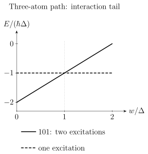
The endpoint interaction is a nonedge term in the intended path graph. Its energy cost can outweigh the reward for the second excitation. The plot assumes zero drive, positive interactions, and $U>\Delta$; it compares the lowest independent configurations. At the crossing, both cardinalities are degenerate.

Even if the final ground state encodes the desired answer, a finite-time ramp need not prepare it. Small gaps, imperfect initial states, noise, and nonadiabatic transitions determine the measured success probability. An encoding theorem is not a runtime guarantee.

Gate fidelity is not a probability that no fault occurred

Suppose a deliberately simplified model assigns each operation an independent classical fault probability $p$. For $G$ operations,

$$P_{\rm no\ fault}=(1-p)^G,\qquad \mathbb E[K]=Gp.$$

These expressions concern the assumed fault process. They cannot generally be evaluated by replacing $1-p$ with a measured average gate fidelity. Average fidelity is an overlap averaged over inputs; it does not specify the noise channel. Faults can also cancel, commute with the observable, or be corrected, so the probability of no faults is not the same as the probability of a correct final answer.

For example, take a coherent unwanted rotation $U_\epsilon=e^{-i\epsilon Z/2}$ applied repeatedly to $|+\rangle$. After $G$ repetitions, the probability to obtain the wrong result in an $X$ measurement is

$$p_X^{\rm coh}=\sin^2(G\epsilon/2).$$

For independent stochastic $Z$ flips with probability $p=\sin^2(\epsilon/2)$ per operation, the same measurement gives

$$p_X^{\rm stoch}=\frac{1-(1-2p)^G}{2}.$$

Both channels have the same single-step average fidelity to the identity, $F_{\rm avg}=1-2p/3$. Nevertheless, at small accumulated error their measurement errors scale as $G^2\epsilon^2/4$ and $G\epsilon^2/4$, respectively. A scalar fidelity alone cannot predict circuit behavior. Fidelity defines the different overlap measures; neutral-atom qubits connects noise models to processor design.

Erasure flags provide location information

For a normalized qubit state, the ideal erasure channel is

$$\mathcal E_\epsilon(\rho) =(1-\epsilon)\rho+\epsilon|e\rangle\langle e|,$$

where $|e\rangle$ is orthogonal to the qubit space. The flag announces loss of the encoded state; it does not reveal its unknown amplitudes or restore them. Quantum error correction can use the location information along with redundancy in the code.

Atomic level structure can make some leakage events detectable, as demonstrated by Scholl et al. (2023). Real detection also has missed events, false flags, delays, and possible disturbance of neighboring atoms. State-dependent survival can even change the state in accepted trials. The ideal channel above assumes a state-independent erasure probability.

For a code of distance $d$, any pattern of fewer than $d$ known-location erasures is correctable in the ideal code-capacity setting. Arbitrary unknown-location errors are guaranteed correctable only up to $\lfloor(d-1)/2\rfloor$. Some larger special patterns may also be correctable; distance gives worst-case guarantees. Faulty syndrome extraction, time-dependent noise, and correlations require a circuit-level analysis. The surface code and erasure channels develop these distinctions.

Suppression with code size is a measured relationship

A commonly used low-noise heuristic for odd-distance codes under suitable local stochastic errors is

$$p_L(d)\approx A\left(\frac{p}{p_{\rm th}}\right)^{(d+1)/2}.$$

Here $p_L$ refers to a specified logical operation or correction cycle. The exponent, prefactor, and threshold depend on the code, circuit, noise, and decoder; the expression is not a universal formula for mixed erasure and coherent errors.

An observed suppression ratio $\Lambda=p_L(d)/p_L(d+2)$ is a directly defined comparison. Identifying it with $p_{\rm th}/p$ additionally assumes the displayed model and a common prefactor. A fitted $\Lambda>1$ does not independently measure every physical error probability. Repeated rounds and comparable operating conditions are needed to learn whether protection continues to improve.

Many-body observables test the physical model

An analog experiment asks about observables under a specified Hamiltonian and preparation. Local densities, connected correlations, excitation statistics, and nonlocal string observables probe different features. Agreement in a mean density does not determine the full quantum state.

Useful comparisons include exact calculations for small systems, tensor networks where entanglement remains manageable, controlled limiting cases, and independently varied geometry or detuning. A parameter fitted to one observable should be tested against others. Computational many-body methods explains the strengths and limitations of the main numerical approaches.

Finite arrays can show ordering, critical behavior, or topological signatures without directly realizing an infinite-system thermodynamic limit. Size dependence, boundary effects, preparation, and readout affect that inference. This is a physical reason to compare several observables and sizes, rather than treating a visually ordered image as a complete phase identification.

For optimization, the measured per-run probability $p_s$ of reaching the specified solution quality enters the cost of repetition. With independent identical attempts, achieving at least one success with probability $q$ requires

$$N_{\rm run}= \left\lceil\frac{\ln(1-q)}{\ln(1-p_s)}\right\rceil, \qquad 0<p_s<1,\quad0<q<1.$$

Preparation, movement, measurement, reset, and classical tuning contribute to elapsed time alongside coherent evolution. Comparisons with classical algorithms should use the same instance distribution and solution quality. Neither an atom count nor the failure of one numerical method alone establishes an advantage.

Exercises

1. Independent gate faults

A layer contains 30 disjoint two-qubit gates. In an illustrative independent stochastic model, each gate has fault probability $p=0.005$.

1. What is the probability that the layer contains no gate fault?
2. What is the probability that a 100-layer circuit contains no gate fault?
3. What is the expected number of gate faults in the 100-layer circuit?

Solution

For one layer,

$$P_{\mathrm{layer}} =(0.995)^{30} \approx 0.860.$$

There are $G=30\times100=3000$ gates in the full circuit, so

$$P_{\mathrm{circuit}} =(0.995)^{3000} \approx 2.95\times10^{-7}.$$

The expected number of faults is

$$\mathbb E[K] =Gp =3000(0.005) =15.$$

This is not a prediction for a fault-tolerant circuit, which detects and corrects faults, nor does it describe coherent or correlated errors. It shows how even a small per-operation fault probability can matter in a long circuit. It does not convert a reported average gate fidelity into $p$.

2. Why the graph Hamiltonian encodes independence

Consider

$$\frac{H}{\hbar} =-\Delta\sum_{i\in V}n_i +U\sum_{(i,j)\in E}n_i n_j, \qquad U>\Delta>0.$$

Show that no ground-state bit string can occupy both endpoints of an edge. Then show that among independent sets, a ground state has maximum cardinality.

Solution

Suppose a configuration occupies both endpoints of at least one edge. Choose an occupied vertex $i$ that has $k\ge1$ occupied neighbors and set $n_i$ from one to zero. Removing the vertex loses the reward $-\Delta$, increasing the first term by $\Delta$, but removes $k$ penalties, decreasing the second term by $kU$. The energy change is

$$\frac{\Delta E}{\hbar} =\Delta-kU \le \Delta-U <0.$$

The original configuration was therefore not a ground state. Every ground state is an independent set.

For an independent set $S$, the penalty term vanishes and

$$E(S)=-\hbar\Delta |S|.$$

Minimizing energy is equivalent to maximizing $|S|$. Thus the ground-state configurations encode maximum independent sets. The argument establishes the static encoding, not the probability that a finite-time quantum evolution finds a ground state.

3. Missed erasures

Each of $n=100$ operations produces an erasure with probability $\epsilon=0.002$. A detector flags a true erasure with efficiency $q=0.98$. Neglect false flags and correlations.

1. What is the probability of at least one physical erasure?
2. What is the per-operation probability of an unflagged erasure?
3. What is the probability of at least one unflagged erasure?

Solution

The probability of at least one erasure is

$$P_{\ge1} =1-(1-\epsilon)^n =1-(0.998)^{100} \approx 0.181.$$

The unflagged probability per operation is

$$\epsilon_{\mathrm{miss}} =\epsilon(1-q) =0.002(0.02) =4.0\times10^{-5}.$$

Hence

$$P_{\mathrm{miss},\ge1} =1-(1-\epsilon_{\mathrm{miss}})^{100} \approx 3.99\times10^{-3}.$$

Efficient flagging converts a common unknown-location event into a much rarer unflagged event, but it does not remove the flagged erasures. The code still needs enough erasure tolerance, and a complete model must add false flags and correlations.

4. A suppression ratio without a threshold inference

Suppose comparable distance-three and distance-five experiments have $p_L(3)=0.02$ and $p_L(5)=0.01$. Find $\Lambda$. If the same suppression continues from distance five to seven, estimate $p_L(7)$. What additional assumption is needed to infer $p/p_{\rm th}$?

Solution

$\Lambda=2$, and the extrapolated $p_L(7)$ is $0.005$. The estimate assumes the same distance-to-distance ratio; it is not a measurement at distance seven. To infer $p/p_{\rm th}=1/2$, one additionally assumes $p_L(d)=A(p/p_{\rm th})^{(d+1)/2}$ with common $A$ and a meaningful single noise parameter $p$. Different noise mixtures or finite-size corrections can give the same observed ratio without that interpretation.

References

• Ebadi, S., et al. “Quantum optimization of maximum independent set using Rydberg atom arrays.” Science 376, 1209–1215 (2022). doi:10.1126/science.abo6587.
• Saffman, M., Walker, T. G., and Mølmer, K. “Quantum information with Rydberg atoms.” Reviews of Modern Physics 82, 2313–2363 (2010). doi:10.1103/RevModPhys.82.2313.
• Scholl, P., Shaw, A. L., Tsai, R. B.-S., Finkelstein, R., Choi, J., and Endres, M. “Erasure conversion in a high-fidelity Rydberg quantum simulator.” Nature 622, 273–278 (2023). doi:10.1038/s41586-023-06516-4.