Precision AMO Frontiers

Precision AMO experiments translate small changes in a field, frequency, or acceleration into quantum phases and measured populations. Their performance depends on more than the smallest reported noise: interrogation time, contrast, bandwidth, repetition rate, calibration, and the interpretation of the signal all matter. This page explains these established relationships and how to compare sensors under the same conditions.

For dated measurements, unresolved questions, and possible research projects, see Precision AMO tests. The calculations below are idealized examples, not forecasts for a particular instrument.

Required background. Precision metrology introduces uncertainty and measurement models. Ramsey interferometry explains phase-to-population conversion, and Fisher information provides the local estimation bound used below.

A sensor responds within a frequency band

For small perturbations about a calibrated operating point, a linear sensor can be described by a signal response, unwanted responses, and noise. If the response is also time invariant, channel $i$ has the frequency-domain form

$$\widetilde y_i(f)=H_{i\theta}(f)\widetilde\theta(f) +\sum_jH_{ij}(f)\widetilde x_j(f)+\widetilde n_i(f).$$

Here $\theta$ is the quantity to be estimated, $x_j$ are environmental or control inputs, and $n_i$ is residual noise. The transfer function $H$ tells you both how strongly and with what phase the sensor responds. For pulsed, time-varying, or nonlinear measurements, use the corresponding two-time response kernel or full measurement model instead of assuming a convolution. Degen, Reinhard, and Cappellaro (2017) develop this way of comparing quantum sensors.

Device	Simple response and its conditions
Atomic magnetometer	$\omega_L=\gamma B$ for the chosen Zeeman manifold and field regime; the response also depends on pumping, relaxation, and measurement bandwidth.
Clock	Detuning accumulates a phase during interrogation; the final population depends on that phase, contrast, and readout.
Light-pulse accelerometer	$\phi_a=\mathbf k_{\mathrm{eff}}\cdot\mathbf a\,T^2$ for the ideal three-pulse sequence with constant acceleration and negligible pulse duration.
Frequency-ratio comparison	Different transitions respond differently to dimensionless constants and environmental shifts.

These scale factors are not complete instruments. Spatial averaging, field gradients, propagation delays, state preparation, and detection can modify the measured response.

Ramsey interrogation as a simple filter

Suppose a weak parameter $\theta(t)$ shifts an angular frequency by $g\theta(t)$, with constant coupling $g$. Neglect pulse duration and decay for the moment. A Ramsey free-evolution interval from $0$ to $T$ accumulates

$$\phi(T)=g\int_0^T\theta(t)\,dt.$$

For a complex harmonic input $\theta(t)=\theta_0e^{i2\pi ft}$, whose real part is the physical signal, the phase amplitude is $H_T(f)\theta_0$, with

$$H_T(f)=gT e^{i\pi fT}\operatorname{sinc}(\pi fT), \qquad \operatorname{sinc}(x)=\frac{\sin x}{x}.$$

At zero frequency $|H_T|=|g|T$: longer interrogation amplifies a static signal. But the first zero moves to $f=1/T$. A signal that completes one full cycle during the interval contributes zero net phase, regardless of its instantaneous amplitude.

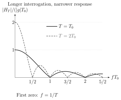
The exact ideal-filter magnitudes $|H_T(f)|/(|g|T_0)$ for $T=T_0$ and $T=2T_0$. Doubling the interval doubles the static response and halves the frequency of the first zero. The curves describe phase accumulation before decoherence, sampling between shots, or detection noise is included.

An echo or a sequence of control pulses changes the sign or weighting of the integrand and can select an oscillatory signal instead. The corresponding sensitivity function is the natural starting point for comparing protocols at the frequency of interest.

Information per unit time

For a regular one-parameter statistical model and a locally unbiased estimator, $\nu$ independent repetitions obey

$$\operatorname{Var}(\hat\theta)\geq\frac{1}{\nu F_C} \geq\frac{1}{\nu F_Q}.$$

$F_C$ is the Fisher information in the chosen measurement, while $F_Q$ is the maximum permitted by the prepared state. A state with large $F_Q$ is helpful only when the readout accesses that information. Pezzè et al. (2018) explain this connection for entangled atomic ensembles.

If each cycle lasts $T_c$, independent repeated measurements have asymptotic information rate $F_C/T_c$. Preparation, cooling, readout, and calibration time count alongside interrogation. Unknown systematic bias is not removed by this statistical bound; correlated cycles require a joint noise model.

A longer interrogation can reduce the information rate

For $N$ independent ideal two-state probes measured at the steepest point of a Ramsey fringe, let the contrast be $C(T)=e^{-T/T_2}$. The binary-outcome Fisher information for a static $\theta$ is

$$F_C(T)=N g^2T^2e^{-2T/T_2}.$$

With dead time $T_d$, the rate is

$$\dot F_C(T)=\frac{N g^2T^2e^{-2T/T_2}}{T+T_d}.$$

If $T_d=0$, differentiating its logarithm gives $1/T-2/T_2=0$, so the optimum is $T=T_2/2$. For nonzero $T_d$, the stationary condition is $2/T-2/T_2-1/(T+T_d)=0$. This is an example under fixed $N$ and exponential contrast decay, not a universal optimum. Technical noise and a different signal waveform change it.

Accepted trials are only part of the experiment

If a fraction $p$ of attempts is accepted independently of $\theta$, and rejected trials contain no useful information, the rate from accepted trials is $pF_{C,\mathrm{acc}}/T_c$. Quoting only the information per accepted trial can hide a low success probability.

When acceptance itself depends on $\theta$, the accept/reject record carries information. For a resolved binary selection flag, the full classical information per attempted trial decomposes as

$$F_{C,\mathrm{full}}= \frac{[\partial_\theta p]^2}{p(1-p)} +pF_{C,\mathrm{acc}}+(1-p)F_{C,\mathrm{rej}}, \qquad 0<p<1.$$

This follows by factoring the joint probability into the flag probability and the conditional outcome distribution. Conditional scores have zero mean, so their cross terms vanish. A valid comparison uses the same total resources and specifies which records are retained.

Calibration and correlated measurements

Separate fluctuations of repeated data from uncertainty in corrections and in the physical response model. When contributions are uncorrelated, their standard uncertainties can be added in quadrature. Shared references, constants, or environmental corrections instead produce covariance.

For example, two measurements with equal variance $u^2$ and correlation $\rho$ have

$$u_{\mathrm{mean}}^2=\frac{u^2}{2}(1+\rho), \qquad u_{\mathrm{difference}}^2=2u^2(1-\rho).$$

Positive correlation weakens the improvement from averaging but can help a difference reject common noise. Whether that also rejects the desired signal depends on its response in the two channels.

Clock comparisons and closure

For three positive frequency ratios with directions $R_{AB}=\nu_A/\nu_B$, $R_{BC}=\nu_B/\nu_C$, and $R_{CA}=\nu_C/\nu_A$, consistency requires

$$\ln R_{AB}+\ln R_{BC}+\ln R_{CA}=0.$$

This is a useful experimental test only when at least one ratio is measured independently. Defining the third ratio from the other two makes closure an algebraic identity. Include shared-oscillator and transfer-link covariances when assigning an uncertainty to the closure residual. Measurements taken at different times also require a model for actual frequency changes.

Optical clocks and Ludlow et al. (2015) explain the clock-specific corrections. Near Earth’s surface, the weak-field relation $\Delta\nu/\nu\simeq g\Delta h/c^2$ gives a fractional shift near $1.1\times10^{-19}$ per millimetre. That conversion alone does not establish millimetre height resolution: averaging time, transfer uncertainty, and the geopotential model still matter.

Phase sensitivity and dynamic range

The atom-interferometer scale factor grows as $T^2$, but the phase is periodic. For a one-axis accelerometer the acceleration change producing $2\pi$ phase is $2\pi/(k_{\mathrm{eff}}T^2)$. A population measurement of a cosine fringe has additional within-period ambiguities unless a second quadrature, a prior, or a lock identifies the operating branch.

Increasing $T$ can therefore improve local sensitivity while making it harder to follow a rapidly changing acceleration. An auxiliary accelerometer, different interrogation times, or adaptive phase control can help identify the fringe. Cronin, Schmiedmayer, and Pritchard (2009) develop the interferometer response; atom-interferometric sensors connects it to practical noise and corrections.

From a measured shift to an interaction

Many precision tests use a linearized response matrix

$$\mathbf y=A\mathbf c+\boldsymbol\epsilon,$$

where $\mathbf c$ contains unknown interaction coefficients and $A$ combines atomic, molecular, nuclear, and instrument responses. The rank of $A$ determines which combinations are identifiable. Almost parallel response columns can leave large uncertainty in individual coefficients even when the measured combinations are precise. Setting all but one coefficient to zero is an additional model assumption.

A spin-independent Yukawa modification is one illustrative parameterization:

$$V(r)=-\frac{Gm_1m_2}{r}\left(1+\alpha_Ye^{-r/\lambda}\right), \qquad \lambda=\frac{\hbar}{m_bc}.$$

$\alpha_Y$ describes a strength relative to gravity for the specified sources. Composition-dependent or spin-dependent forces require their own charges and operators. The range alone does not determine a detector’s response: source geometry, gradients, and shielding or screening assumptions can matter.

Likewise, a bound on an oscillation of a dimensionless constant is not yet a bound on every dark-matter model. The conversion to field coupling may require the field density and coherence. Those assumptions are distinct from the measured frequency-ratio limit itself. Safronova et al. (2018) develop these interpretations; fundamental symmetry tests and variation-of-constants searches give the relevant AMO response models.

Choosing a comparison

For a useful comparison, hold the physical task fixed. A static magnetic field, a known-frequency oscillation, and an unknown transient require different estimators. State the observation time, accepted frequency band, total cycle time, particle or photon resources, and environmental conditions.

Then compare the quantity that answers the question: an uncertainty after a specified time, a frequency-dependent detection probability, or a model-bound curve with a stated coverage procedure. A low amplitude spectral density in one band does not establish a low uncertainty for all waveforms. Reversing a field or comparing two sensors can isolate a response symmetry, but an unwanted effect can have that same symmetry.

For research directions and measurements with their publication dates, use Precision AMO tests. The experimental implementations are developing; the transfer functions, statistical assumptions, and limiting calculations above explain what those developments must be compared against.

Exercises

1. Information rate, not single-shot gain

Protocol A uses uncorrelated atoms, has Fisher information $F_A=1.0\times10^4$ per shot, and cycles every $1.0\ \mathrm{s}$. Protocol B uses a squeezed state, has $F_B=2.5\times10^4$ per accepted shot, takes $2.0\ \mathrm{s}$ per attempted cycle, and accepts $80\%$ of attempts. Assume the acceptance probability is parameter independent, rejected shots contain no information, and the measurements attain their classical Cramér–Rao bounds in the repeated-trial limit.

1. Compute the Fisher-information rate for each protocol.
2. Which has the smaller ideal statistical variance after one hour?
3. By what factor?

Solution

For A,

$$\dot F_A = \frac{10^4}{1.0\ \mathrm{s}} = 1.0\times10^4\ \mathrm{s}^{-1}.$$

For B, the accepted information per attempt is $0.80F_B=2.0\times10^4$, so

$$\dot F_B = \frac{2.0\times10^4}{2.0\ \mathrm{s}} = 1.0\times10^4\ \mathrm{s}^{-1}.$$

The protocols have equal ideal information rate and therefore equal Cramér–Rao variance after one hour. Protocol B has a single-shot resource gain but no wall-clock statistical gain under the stated overhead. Their systematic errors and dynamic ranges would still need comparison.

2. Atom-interferometer scale and phase ambiguity

An ideal light-pulse accelerometer has $k_{\mathrm{eff}}=1.61\times10^7\ \mathrm{m}^{-1}$ and $T=0.20\ \mathrm{s}$.

1. Find the phase change caused by $\delta a=1.0\times10^{-8}\ \mathrm{m\,s^{-2}}$.
2. Find the acceleration interval corresponding to a $2\pi$ phase change.
3. Explain why sensitivity and dynamic range must be reported together.

Solution

Using $\delta\phi=k_{\mathrm{eff}}\delta aT^2$,

$$\delta\phi = (1.61\times10^7) (1.0\times10^{-8}) (0.20)^2 = 6.44\times10^{-3}\ \mathrm{rad}.$$

One $2\pi$ period corresponds to

$$\Delta a_{2\pi} = \frac{2\pi} {k_{\mathrm{eff}}T^2} \approx 9.76\times10^{-6}\ \mathrm{m\,s^{-2}}.$$

Increasing $T$ amplifies a small acceleration but shrinks the phase-period acceleration interval as $T^{-2}$. A cosine population measurement also needs a known branch or phase quadrature. A high-sensitivity interferometer may need a chirp, midfringe lock, auxiliary accelerometer, multiple scale factors, or phase-unwrapping model in a dynamic environment.

3. Correlated clock-network uncertainty

Two clock ratios $r_1$ and $r_2$ each have standard uncertainty $u=3.0\times10^{-18}$ and correlation coefficient $\rho=0.60$ because they share an oscillator and link. Find the standard uncertainty of:

1. the average $(r_1+r_2)/2$;
2. the difference $r_1-r_2$.

Treat the ratios as small fractional deviations around nominal values.

Solution

The covariance is $\operatorname{Cov}(r_1,r_2)=\rho u^2$. Therefore

$$\operatorname{Var} \left( \frac{r_1+r_2}{2} \right) = \frac{u^2+u^2+2\rho u^2}{4} = \frac{u^2}{2}(1+\rho).$$

Thus

$$u_{\mathrm{avg}} = 3.0\times10^{-18} \sqrt{0.8} \approx 2.68\times10^{-18}.$$

For the difference,

$$\operatorname{Var}(r_1-r_2) = 2u^2(1-\rho),$$

so

$$u_{\mathrm{diff}} = 3.0\times10^{-18} \sqrt{0.8} \approx 2.68\times10^{-18}.$$

The equal numerical values are specific to $\rho=0.60$. Positive common-mode correlation weakens averaging but improves a difference relative to the uncorrelated case.

4. Noise spectral density and integration

A magnetometer has one-sided white magnetic-noise amplitude $S_B^{1/2}=15\ \mathrm{fT}/\sqrt{\mathrm{Hz}}$ over the relevant band. For a known-phase sinusoidal signal spanning many periods, with unity calibrated response and an ideal matched estimator, estimate the statistical amplitude uncertainty after $\tau=400\ \mathrm{s}$ using $u_B\simeq S_B^{1/2}/\sqrt{\tau}$. Why is this not automatically a detection limit for an unknown-frequency signal?

Solution

The ideal uncertainty is

$$u_B \simeq \frac{15\ \mathrm{fT}/\sqrt{\mathrm{Hz}}} {\sqrt{400\ \mathrm{s}}} = 0.75\ \mathrm{fT}.$$

An unknown-frequency search scans multiple frequencies, phases, and possibly time windows. It must account for the spectral window, nonwhite noise, calibration, line broadening, trials factor, and detection efficiency. Environmental lines can also occupy the same band. The one-template uncertainty is therefore not a global discovery threshold.

References

• A. D. Cronin, J. Schmiedmayer, and D. E. Pritchard, “Optics and interferometry with atoms and molecules,” Reviews of Modern Physics 81, 1051–1129 (2009).
• C. L. Degen, F. Reinhard, and P. Cappellaro, “Quantum sensing,” Reviews of Modern Physics 89, 035002 (2017). A platform-spanning account of quantum-sensor protocols, sensitivity, and noise.
• A. D. Ludlow, M. M. Boyd, J. Ye, E. Peik, and P. O. Schmidt, “Optical atomic clocks,” Reviews of Modern Physics 87, 637–701 (2015).
• L. Pezzè, A. Smerzi, M. K. Oberthaler, R. Schmied, and P. Treutlein, “Quantum metrology with nonclassical states of atomic ensembles,” Reviews of Modern Physics 90, 035005 (2018). The standard entry point for entanglement-assisted atomic metrology.
• M. S. Safronova et al., “Search for new physics with atoms and molecules,” Reviews of Modern Physics 90, 025008 (2018).