Photon Sources, Nonclassical Light, and Optical Memories

Quantum-optical experiments connect a prepared field to a measurement through interferometers, channels, and sometimes quantum memories. The useful resource must survive that whole path. A source can emit very clean single photons infrequently; a circuit can process its surviving photons accurately while losing most of them. Understanding both the state and the probability of obtaining it is essential.

This page connects the basic optical models to source design, photonic processing, and elementary network links. Dated experimental results and open research questions are collected in Quantum optics frontiers.

Required background. The quantum-optics overview introduces states and modes; photon counting explains detector outcomes; squeezed light and parametric down-conversion introduce the optical resources used below. Continuous-variable systems supplies the quadrature language.

A single photon must occupy a useful mode

A normalized wavepacket has creation operator

$$a_f^\dagger=\int d\omega\,f(\omega)a^\dagger(\omega), \qquad \int d\omega\,|f(\omega)|^2=1.$$

Spatial shape and polarization must also be specified. Two sources can each emit exactly one photon yet fail to interfere because those modes are different. Filtering can improve their overlap, but it usually reduces the probability of delivering a photon.

For independent single-photon inputs with internal-mode density matrices $\rho_1,\rho_2$, a balanced, lossless beam splitter followed by detectors that collect all the relevant output modes gives

$$P_{\mathrm{coinc}}=\frac{1-\operatorname{Tr}(\rho_1\rho_2)}{2}.$$

The distinguishable reference has coincidence probability $1/2$, so the Hong–Ou–Mandel visibility is $\operatorname{Tr}(\rho_1\rho_2)$ under these assumptions. In particular, two independently prepared copies of the same mixed mode give visibility $\operatorname{Tr}(\rho_1^2)$, which need not be one. Correlations between inputs, multiphoton events, unbalanced splitting, mode-dependent loss, or selective time windows require a different measurement model. See beam splitters for the two-photon calculation.

Photon number, brightness, and overlap answer different questions

For a specified pulse mode with nonzero mean occupation,

$$g^{(2)}=\frac{\langle n(n-1)\rangle}{\langle n\rangle^2}.$$

This is a number-statistics quantity. It is not automatically the same as every experimentally plotted zero-delay correlation: time binning and the receiver response matter. Consider

$$\rho=(1-p)|0\rangle\langle0|+p|1\rangle\langle1|, \qquad 0<p\leq1.$$

It has $g^{(2)}=0$ for every $p$, including very small $p$. Thus a small correlation value does not determine the delivery probability. It also says nothing about whether the one-photon wavepacket matches a second source.

For a source with at most one photon per pulse, delivery probability $p$, repetition frequency $f$, and detector efficiency $\eta_d$, the unsaturated count rate is $fp\eta_d$. For a general source, $f\eta_d\langle n\rangle$ is instead the mean detected photon number per unit time in an ideal linear receiver; a threshold detector counts clicks and can give a different rate. Lodahl, Mahmoodian, and Stobbe (2015) discuss how emitter coupling, collection, and mode quality enter single-photon sources.

A herald click changes the photon-number distribution

In an ideal, single-Schmidt-mode pair source, the signal and idler share the geometric pair distribution

$$P_n=(1-q)q^n,\qquad \mu=\frac{q}{1-q},\qquad 0<q<1.$$

An ideal threshold herald clicks whenever $n\geq1$. Its multipair fraction is then $P(n\geq2\mid\mathrm{click})=q$. Increasing pump strength raises both the herald rate and the unwanted multipair contribution.

Now suppose each idler photon is detected independently with probability $0<\eta_h\leq1$, and the herald detector has no dark counts or number resolution. For $n$ pairs, its click probability is

$$c_n=1-(1-\eta_h)^n.$$

Bayes’ rule gives the actual conditioned distribution:

$$P(n\mid\mathrm{click})=\frac{P_n c_n}{P_{\mathrm{click}}}, \qquad P_{\mathrm{click}}=\frac{q\eta_h}{1-q+q\eta_h}.$$

In particular,

$$\begin{aligned} P(1\mid\mathrm{click})&=(1-q)(1-q+q\eta_h),\\ P(n\geq2\mid\mathrm{click})&=1-(1-q)(1-q+q\eta_h). \end{aligned}$$

Inefficient heralding favors larger pair numbers because they have more chances to trigger the detector. This is why replacing a real click by the ideal condition “at least one pair was created” can underestimate contamination.

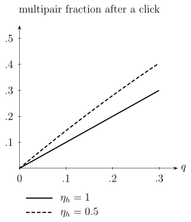
The same pair source produces different conditional ensembles when the herald detector changes. The curves assume one pair mode, threshold detection, independent losses, and no dark counts; signal-arm loss has not yet been applied.

Loss after heralding can leave vacuum in the signal arm. A dark herald can also accept a vacuum trial. Number-resolving detection changes the weighting $c_n$, but inefficient number resolution can still mistake several emitted photons for one detected photon. For multimode sources, sum over the appropriate joint mode occupations rather than assuming the geometric single-mode distribution. The underlying state is derived in parametric down-conversion.

Multiplexing trades more attempts for routing loss

For $M$ independent, identical attempts with success probability $p$,

$$P_{\geq1}=1-(1-p)^M.$$

If a balanced binary tree with $M=2^d$ routes one selected photon through $d$ switches, each with transmission $\tau$, a simplified delivery model is

$$P_{\mathrm{del}}=[1-(1-p)^M]\tau^d.$$

The assumptions are significant: each accepted source supplies a suitable photon, the controller chooses one success correctly, all selected paths have the same loss, and delays and other interfaces are ideal. Unbalanced trees and temporal multiplexers can have path-dependent storage loss. Increasing $M$ makes a herald more likely, but need not indefinitely improve delivery once routing, storage, and source correlations are included.

Loss and phase noise limit useful squeezing

Use $X_\theta=(ae^{-i\theta}+a^\dagger e^{i\theta})/\sqrt2$, whose vacuum variance is $1/2$. Write the measured variance relative to vacuum as $R=2\operatorname{Var}X_\theta$. For a pure squeezed vacuum with parameter $r\geq0$, the principal variance ratios are $e^{-2r}$ and $e^{2r}$.

If the measurement axis fluctuates by an independent, zero-mean Gaussian angle $\delta$ of variance $\sigma^2$, the averaged input variance ratio is

$$\begin{aligned} \overline R &=e^{-2r}\langle\cos^2\delta\rangle +e^{2r}\langle\sin^2\delta\rangle\\ &=\cosh(2r)-e^{-2\sigma^2}\sinh(2r). \end{aligned}$$

Pure loss of transmissivity $\eta$, with vacuum in the unused port, then gives

$$R_{\mathrm{out}}=1-\eta+\eta\overline R.$$

This model neglects technical excess noise and assumes fixed squeezing strength. It shows two different mechanisms. Loss mixes in vacuum; phase jitter mixes the large anti-squeezed variance into the measured quadrature. For nonzero $\sigma$, the optimum is finite:

$$\tanh(2r_{\mathrm{opt}})=e^{-2\sigma^2}.$$

The result follows by differentiating $\overline R$ with respect to $r$. With perfect phase control the optimum moves toward arbitrarily large $r$, but loss still imposes the limiting ratio $1-\eta$. Positive squeezing in decibels is defined here as $S=-10\log_{10}R_{\mathrm{out}}$.

An inferred source variance obtained by correcting for known loss is useful for characterizing the source. The receiver operates with the variance after that loss. The detailed optical transformations are developed in squeezed light; Gaussian loss channels are discussed by Weedbrook et al. (2012).

Gaussian operations and non-Gaussian resources

Gaussian states are described by means and covariance matrices. Quadratic Hamiltonians, Gaussian channels, and ideal homodyne or heterodyne measurements permit efficient calculations with those quantities. This includes large entangled Gaussian states; entanglement alone does not make their Gaussian measurement statistics hard to simulate.

An exact homodyne result leaves the remaining conditional state Gaussian. Ignoring a result after nonlinear feed-forward, or accepting a broad non-Gaussian region of outcomes, can instead produce a non-Gaussian mixture. That observation does not bypass the efficient sampling description: one can sample the underlying Gaussian outcomes and apply the classical rule. Rare acceptance can be costly for both the experiment and the simulation.

Photon counting or a non-Gaussian input can take a circuit outside the Gaussian state-and-measurement setting. This does not by itself prove a computational advantage. A sampling experiment asks for a particular distribution; universal computation and fault tolerance require additional operations and error control. See photonic qubits for the computational architectures.

Non-Gaussianity, Wigner negativity, and fault tolerance are also different properties. A mixture of two separated coherent states is generally non-Gaussian while retaining a nonnegative Wigner function. A negative Wigner function diagnoses a stronger feature, but says nothing by itself about how frequently the state is prepared or how accurately a logical operation works. Phase-space distributions explains these distinctions; Weedbrook et al. (2012) gives the broader continuous-variable framework.

A network must wait for random successes

For fibre attenuation $\alpha$ in decibels per kilometre and distance $L$ in kilometres, the channel transmission is

$$\eta_{\mathrm{ch}}=10^{-\alpha L/10}.$$

In a two-photon midpoint protocol, each photon travels $L/2$. The probability that both survive the fibre is $\eta_{L/2}^2=\eta_L$, not $\eta_L^2$. Emission, coupling, conversion, detector response, and Bell-measurement acceptance further affect success. Interference visibility generally changes the conditional output state; it is not a universal extra multiplicative success factor.

Suppose an elementary link succeeds independently with probability $p$ per attempt of duration $T_c$. The number of attempts $N=1,2,\ldots$ is geometric:

$$\Pr(N=n)=p(1-p)^{n-1},\qquad \langle N\rangle=\frac1p.$$

The mean creation time is $T_c/p$. The cycle must include whichever preparation, reset, and communication delays the actual protocol requires. Two neighboring links attempted in parallel and stored after success have

$$\langle\max(N_1,N_2)\rangle =\frac2p-\frac1{p(2-p)}.$$

To obtain this, use $\max+\min=N_1+N_2$. The minimum is geometric with success probability $1-(1-p)^2=p(2-p)$. At small $p$, the mean time for both links is about $3T_c/(2p)$, even before swapping.

The earlier link waits for the later one. Memory decay depends on the distribution of that waiting time, not just its mean: in general $\langle e^{-T/T_2}\rangle\ne e^{-\langle T\rangle/T_2}$. Here $T_2$ describes the coherence of the stored state; it need not equal a single constituent qubit’s measured coherence time. Quantum repeaters derives the exact average for this two-link model and connects it to the fidelity after an ideal entanglement swap. Finite memory lifetimes, cutoffs, repeated swaps, and unequal links require a fuller stochastic model. Sangouard et al. (2011) develops these issues for repeaters based on atomic memories and optical measurements.

A secret-key link, an entangled memory pair, and a repeater serve different tasks. Repeater comparisons must hold the endpoints, allowed intermediate resources, channel uses, and desired output fixed. Otherwise an improved rate can simply reflect a different communication problem.

Exercises

1. A real herald detector

A single-mode pair source has $q=0.05$ and herald efficiency $\eta_h=0.5$. Find the click probability and the multipair fraction among clicks. Compare with an ideal herald.

Solution

The click probability is $0.025/0.975=0.025641$. The conditional one-pair probability is $(0.95)(0.975)=0.92625$, so the multipair fraction is $0.07375$, or $7.375\%$. An ideal herald gives a $5\%$ click probability and a $5\%$ conditional multipair fraction. Lower efficiency both reduces the herald rate and changes the selected ensemble.

2. Routing losses

Take $M=32$ independent source bins, each with $p=0.05$, and a five-stage tree with $\tau=0.98$. Find the ideal herald probability and simplified delivery probability. Does every herald now supply a photon?

Solution

$$P_{\geq1}=1-0.95^{32}\simeq0.8063,\qquad P_{\mathrm{del}}=P_{\geq1}(0.98)^5\simeq0.7288.$$

No. The route can lose the selected photon. Source-mode mismatch, herald mistakes, and delay loss can reduce useful delivery further. A herald is information about a preparation event, not immunity to later loss.

3. Why more squeezing can hurt

For $\sigma=0.05$ radians and $\eta=0.9$, calculate $r_{\mathrm{opt}}$ and the minimum output variance ratio. Compare with a $15\,\mathrm{dB}$ pure source at the same phase jitter and transmission.

Solution

Put $c=e^{-2\sigma^2}$. Then

$$r_{\mathrm{opt}}=\frac12\operatorname{artanh}c\simeq1.498, \qquad \overline R_{\min}=\sqrt{1-c^2}\simeq0.09975.$$

The output ratio is $0.1+0.9(0.09975)\simeq0.1898$, or about $7.22\,\mathrm{dB}$ of squeezing. A $15\,\mathrm{dB}$ pure source has $e^{-2r}=10^{-1.5}$ and $e^{2r}=10^{1.5}$. Substitution gives $R_{\mathrm{out}}\simeq0.1994$, or about $7.00\,\mathrm{dB}$. The stronger source performs slightly worse because its anti-squeezed noise is larger.

4. A midpoint link and two waiting memories

Use $\alpha=0.2\,\mathrm{dB/km}$ and endpoint separation $L=100\,\mathrm{km}$. Find the two-photon fibre survival probability. Separately, two equal elementary links have per-attempt success $p=0.01$ and cycle duration $T_c=1\,\mathrm{ms}$. How long, on average, until both have succeeded, assuming perfect storage?

Solution

Each $50\,\mathrm{km}$ half transmits $10^{-1}=0.1$, so the two-photon fibre factor is $0.1^2=0.01$. This is not the full link success probability.

For the two independent links,

$$\langle T_{\mathrm{both}}\rangle =1\,\mathrm{ms}\left(200-\frac1{0.0199}\right) \simeq149.75\,\mathrm{ms}.$$

A single link takes $100\,\mathrm{ms}$ on average. The earlier memory must survive the additional random wait; replacing the two-link process by one mean creation time misses this requirement.

References

• Lodahl, P., Mahmoodian, S., and Stobbe, S. “Interfacing Single Photons and Single Quantum Dots with Photonic Nanostructures.” Reviews of Modern Physics 87, 347–400 (2015). DOI: 10.1103/RevModPhys.87.347.
• Sangouard, N., Simon, C., de Riedmatten, H., and Gisin, N. “Quantum Repeaters Based on Atomic Ensembles and Linear Optics.” Reviews of Modern Physics 83, 33–80 (2011). DOI: 10.1103/RevModPhys.83.33.
• Weedbrook, C., et al. “Gaussian Quantum Information.” Reviews of Modern Physics 84, 621–669 (2012). DOI: 10.1103/RevModPhys.84.621.