Parametric Down-Conversion

Spontaneous parametric down-conversion (SPDC) is a second-order nonlinear optical process in which a pumped medium creates correlated excitations in two lower-frequency field modes. The outgoing photons are conventionally called the signal and idler. In the simplest bookkeeping,

$$\omega_p = \omega_s+\omega_i,$$

and phase matching selects wavevectors and polarizations that add coherently through the device.

SPDC is valuable because one physical interaction can prepare several different resources:

• a time-correlated photon pair;
• a heralded single photon, conditioned on detecting its partner;
• a polarization-, path-, frequency-, orbital-angular-momentum-, or time-bin entangled pair;
• a two-mode squeezed state when more than one pair sector matters.

These outputs are not automatic consequences of writing $\omega_p=\omega_s+\omega_i$. Their quality depends on the pump mode, susceptibility tensor, phase matching, crystal or waveguide geometry, spatial collection, spectral filtering, loss, detector response, and whether unobserved degrees of freedom reveal which creation alternative occurred.

Here spontaneous means that signal and idler enter in vacuum. An incoherent thermal population can also stimulate emission, even though its mean field vanishes. It does not mean that energy or momentum conservation is abandoned, and it does not make the source deterministic. At useful low gain, most pump pulses produce no collected pair; raising the pump also raises unwanted multipair probability.

Required background. Nonlinear quantum optics derives the pair interaction, quantized modes fixes field normalization, photon-number states supplies counting statistics, and Schmidt decomposition explains the mode pairs used below.

Pump Photon Conversion

Selected-mode Hamiltonian

After the pump, spatial modes, polarizations, and nearly resonant frequencies have been selected, with signal and idler in orthogonal modes, the undepleted-pump interaction can reduce to

$$H_I = i\hbar \left( \xi a_s^\dagger a_i^\dagger - \xi^*a_sa_i \right).$$

The complex coupling $\xi$ contains the classical pump amplitude, the relevant component of $\chi^{(2)}$, a mode-overlap integral, a phase-matching factor, and normalization constants. Its phase sets the phase of the created-pair amplitude. This Hamiltonian creates or annihilates signal-idler pairs and conserves the number difference,

$$[H_I,n_s-n_i]=0.$$

Starting from vacuum therefore populates equal-number sectors.

The description “one pump photon splits into two photons” captures the energy bookkeeping, but it should not be read too literally in the usual undepleted-pump model. There the pump is replaced by a prescribed coherent field, so individual pump quanta are not tracked. A fully quantized three-mode Hamiltonian tracks pump depletion and conserves $n_p+n_s$ and $n_p+n_i$, not the pump occupation separately. The classical-pump approximation is excellent for weak conversion from a strong laser field.

Low-gain biphoton limit

For a short or weak interaction, first-order perturbation theory gives

$$|\Psi\rangle \simeq{} |0\rangle + \eta|\psi_2\rangle + O(\eta^2),$$

where $|\psi_2\rangle$ is a normalized two-photon state and $|\eta|^2\ll1$ is the collected pair probability to leading order. A normalized expression must retain the vacuum coefficient; writing only $|\psi_2\rangle$ describes the state conditioned on pair production, not the unconditional optical output.

At low gain, the pair amplitude is linear in pump field amplitude, while the pair probability is linear in pump pulse energy or continuous-wave pump power, provided repetition rate, pulse shape, collection, and phase matching are held fixed. This scaling fails when gain, pump depletion, thermal loading, photorefractive effects, or detector saturation becomes important.

The term $O(\eta^2)$ contains two-pair amplitudes. It cannot be omitted when a protocol is sensitive to false heralds, accidental coincidences, or four-photon events.

Beyond one pair

For one ideal signal-idler mode pair, the exact undepleted-pump state can be written

$$|\Psi\rangle = \sqrt{1-q} \sum_{n=0}^{\infty} q^{n/2}e^{in\phi} |n_s,n_i\rangle,$$

where

$$q=\tanh^2r, \qquad \bar n=\sinh^2r=\frac{q}{1-q}.$$

Its pair-number distribution is geometric:

$$P_n = (1-q)q^n.$$

Thus increasing the mean pair number also increases the relative weight of the $n\ge2$ sectors. A pulsed traveling-wave source generally contains several independent squeezed mode pairs rather than one ideal pair in the pure, lossless, classical-pump description. At high gain their shapes need not equal the low-gain JSA Schmidt modes because of time ordering. The total pair-number distribution then depends on the modal weights and can look less thermal as more weakly occupied modes contribute.

Spontaneous and stimulated operation

With vacuum signal and idler inputs, pair production is spontaneous. Injecting a seed into one output mode stimulates coherent emission into the partner mode; the same device then operates as an optical parametric amplifier or difference-frequency converter, depending on frequencies and selected rotating-wave terms.

Stimulated measurements can efficiently probe parts of the spontaneous transfer function, but a classical intensity measurement alone does not determine every phase or quantum-noise property of the emitted biphoton state. The measurement model must say which complex response is reconstructed.

Energy and Momentum Matching

Energy matching

For a monochromatic stationary pump,

$$\omega_p = \omega_s+\omega_i.$$

In vacuum wavelengths this becomes

$$\frac1{\lambda_p} = \frac1{\lambda_s} + \frac1{\lambda_i}.$$

The relation does not say that signal and idler must have equal frequency. The process is degenerate when $\omega_s=\omega_i=\omega_p/2$ and nondegenerate otherwise.

For a pulsed pump, each pump spectral component still obeys the frequency-sum rule in a stationary medium. Integrating over those components gives the envelope

$$\alpha_p(\omega_s+\omega_i),$$

which weights a band around the central sum frequency. Shorter pump pulses broaden that sum-frequency band for fixed transform-limited pulse shape; chirp can lengthen a pulse without narrowing its spectrum.

Vector phase matching

Efficient buildup also requires the polarization-dependent wavevectors to match:

$$\Delta\mathbf k = \mathbf k_p-\mathbf k_s-\mathbf k_i-\mathbf G \approx 0.$$

Here $\mathbf G$ is zero for ordinary birefringent phase matching and is a reciprocal vector for quasi-phase matching. For a periodically poled device,

$$\mathbf G = \frac{2\pi m}{\Lambda}\,\hat{\mathbf z},$$

where $\Lambda$ is the poling period and $m$ is a present Fourier harmonic. For an ideal 50% duty-cycle sign reversal, only odd harmonics occur, and first-order matching uses an effective coupling $2/\pi$ of the local value. Temperature, angle, wavelength, and polarization change the refractive indices and therefore tune $\Delta\mathbf k$.

Energy matching prevents rapid temporal phase winding. Phase matching makes emission from different positions add coherently. Both are required for an efficient, well-defined source.

Finite interaction length

For a uniform collinear device of length $L$, the longitudinal amplitude is

$$\begin{aligned} \Phi(\Delta k) &= \int_0^L dz\,e^{i\Delta k z} \\ &= L e^{i\Delta kL/2} \operatorname{sinc} \left( \frac{\Delta kL}{2} \right), \end{aligned}$$

with $\operatorname{sinc}x=\sin x/x$. The corresponding intensity envelope is

$$|\Phi(\Delta k)|^2 = L^2 \operatorname{sinc}^2 \left( \frac{\Delta kL}{2} \right).$$

A longer device gives a larger exactly phase-matched amplitude but a narrower phase-matching acceptance. “Longer is brighter” is therefore incomplete: dispersion, focusing, walk-off, absorption, propagation loss, and collection bandwidth can reverse the expected improvement.

Group-velocity structure

Near central frequencies, write

$$\begin{aligned} \omega_s&=\bar\omega_s+\Omega_s, \\ \omega_i&=\bar\omega_i+\Omega_i. \end{aligned}$$

For collinear down-conversion,

$$\Delta k \simeq{} \Delta k_0 + \left( k'_p-k'_s \right)\Omega_s + \left( k'_p-k'_i \right)\Omega_i,$$

where $k'_j=\partial k_j/\partial\omega$ is the inverse group velocity. The pump envelope and phase-matching function therefore occupy different directions in the $(\Omega_s,\Omega_i)$ plane. Group-velocity engineering can make their product nearly factorable; poor alignment produces strong spectral entanglement.

Geometry and polarization types

Several labels answer independent questions:

• Type-0: pump, signal, and idler use the same polarization family.
• Type-I: signal and idler share a polarization, with the pump using a different allowed tensor channel.
• Type-II: signal and idler have orthogonal polarizations.
• Collinear or noncollinear: output wavevectors do or do not share the pump axis.
• Degenerate or nondegenerate: output frequencies are or are not equal.
• Bulk, waveguide, resonator, or integrated: the spatial eigenmodes and density of states differ.

These terms should not be collapsed into one another. A source can be degenerate but noncollinear, Type-II but frequency nondegenerate, or quasi-phase-matched and collinear.

For a focused pump, transverse momentum conservation has a finite width:

$$\mathbf q_s+\mathbf q_i \approx \mathbf q_p,$$

where $\mathbf q$ denotes transverse wavevector. Focusing increases intensity but broadens angular content and can couple spatial and spectral variables. Birefringent spatial walk-off and polarization-dependent group delay can also record which alternative occurred unless compensated.

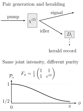
Top: an idler click identifies an event and conditions the signal state; it does not launch the signal photon. Bottom: the two-bin pair amplitude $F_\phi$ has joint probabilities $1/4$ at every phase, but its unresolved heralded purity falls from 1 to $1/2$. Exercise 2 derives the curve.

Signal and Idler Photons

Labels, not a causal order

“Signal” and “idler” are bookkeeping labels inherited from parametric amplification. Either photon may be used as the herald, and neither is fundamentally created first. In a nondegenerate source, the labels are often assigned by wavelength or experimental role. In a degenerate Type-I source, spatial output ports may be the only labels.

If every degree of freedom is identical and both excitations occupy the same mode, the state is a two-photon Fock state of that mode rather than a tensor product of intrinsically named particles. The subsystem decomposition comes from modes, not particle serial numbers.

Biphoton state

Restricting attention to distinct orthogonal signal and idler mode families, the normalized two-photon component is

$$|\psi_2\rangle ={} \int d\omega_s\,d\omega_i \times f(\omega_s,\omega_i) a_s^\dagger(\omega_s) a_i^\dagger(\omega_i) |0\rangle,$$

with

$$\int d\omega_s\,d\omega_i\, |f(\omega_s,\omega_i)|^2 = 1.$$

The joint spectral amplitude (JSA) has the schematic form

$$f(\omega_s,\omega_i) \propto{} \alpha_p(\omega_s+\omega_i) \times \Phi(\omega_s,\omega_i) \mathcal M(\omega_s,\omega_i),$$

where $\mathcal M$ contains polarization, spatial overlap, collection, and normalization factors.

The joint spectral intensity (JSI),

$$\operatorname{JSI}(\omega_s,\omega_i) = |f(\omega_s,\omega_i)|^2,$$

does not reveal the full JSA. Spectral phase can change temporal correlations, the heralded spectral purity, and pulse shape while leaving the JSI unchanged. A separable phase $e^{i\varphi_s(\omega_s)+i\varphi_i(\omega_i)}$ changes local pulse shapes but preserves Schmidt coefficients; nonseparable phase can change the entanglement itself. A claim of complete state characterization from intensity alone therefore requires additional phase assumptions or measurements.

Schmidt modes and heralded purity

A Schmidt decomposition writes

$$\begin{aligned} f(\omega_s,\omega_i) ={}& \sum_k \sqrt{\lambda_k}\, u_k(\omega_s)v_k(\omega_i), \\ \sum_k\lambda_k ={}& 1. \end{aligned}$$

Within a pure one-pair sector, a spectrally uniform unresolved idler herald is equivalent to a partial trace and gives

$$\rho_s = \sum_k \lambda_k |1_{u_k}\rangle \langle1_{u_k}|.$$

The ideal spectral purity and Schmidt number are

$$\begin{aligned} \mathcal P_s &= \operatorname{Tr}(\rho_s^2) = \sum_k\lambda_k^2, \\ K &= \frac1{\sum_k\lambda_k^2} = \frac1{\mathcal P_s}. \end{aligned}$$

A factorable JSA has one nonzero Schmidt coefficient and produces an ideally pure heralded spectral mode. Spectral correlation makes the conditional signal mixed when the herald detector does not resolve the correlated idler mode. A coherent rank-one idler-mode projection instead prepares a pure conditional signal even for an entangled JSA. Spectral resolution followed by forgetting the outcome is not that projection.

Narrow filtering can raise purity by discarding correlated modes, but usually reduces brightness and heralding efficiency. Dispersion and pump engineering can instead rotate and shape the pump and phase-matching functions toward a factorable product. Spatial filtering must be included in this reasoning: spatial-spectral coupling can spoil a calculation that treats only frequency.

Pair timing and correlations

SPDC pairs are produced within a joint temporal amplitude set by pump coherence, phase matching, propagation, and filtering. The historical phrase “simultaneous photons” refers to a narrow relative detection-time correlation after path delays are accounted for. It does not imply two infinitely short wave packets or a perfectly known absolute creation time.

A normalized cross-correlation is

$$g_{si}^{(2)}(0) = \frac{ \langle n_sn_i\rangle }{ \langle n_s\rangle \langle n_i\rangle }.$$

At low brightness it can be very large because pair detections dominate over independent singles. A large cross-correlation certifies strong correlation, not by itself entanglement. Entanglement requires coherence across alternatives and an appropriate witness, tomography, or Bell test.

Polarization Entanglement

Coherent creation alternatives

Polarization entanglement is produced when the source coherently superposes two pair-creation alternatives. A common target family is

$$|\psi_{\rm pol}\rangle ={} \cos\theta |H_sH_i\rangle + e^{i\phi}\sin\theta |V_sV_i\rangle.$$

For $\theta=\pi/4$, the Schmidt coefficients in polarization are equal and the state is maximally entangled, provided no other degree of freedom carries which-alternative information. Type-II geometries often target

$$|\psi_{\rm II}\rangle = \frac{ |H_sV_i\rangle + e^{i\phi}|V_sH_i\rangle }{ \sqrt2 }.$$

The superposition, not the mere presence of orthogonal polarizations, creates entanglement. A source that emits the two alternatives incoherently produces a classical mixture with the same populations in the $H/V$ basis.

Hidden distinguishability

Let $|u\rangle$ and $|v\rangle$ denote all unobserved spectral, spatial, and temporal degrees of freedom associated with two nominal polarization alternatives:

$$|\Psi\rangle = \frac{ |HH\rangle|u\rangle + e^{i\phi}|VV\rangle|v\rangle }{ \sqrt2 }.$$

Define their overlap by

$$\gamma=\langle v|u\rangle.$$

After tracing out the hidden modes,

$$\rho_{\rm pol} = \frac12 \Big( |HH\rangle\langle HH| + |VV\rangle\langle VV| + e^{-i\phi}\gamma |HH\rangle\langle VV| + e^{i\phi}\gamma^* |VV\rangle\langle HH| \Big).$$

Its purity is

$$\operatorname{Tr}(\rho_{\rm pol}^2) = \frac{1+|\gamma|^2}{2}.$$

Perfectly matched hidden modes give $|\gamma|=1$ and preserve polarization coherence. Orthogonal hidden records give $\gamma=0$ and erase the off-diagonal terms. Compensation plates, pump shaping, narrow collection modes, and spectral engineering are therefore part of the state preparation, not cosmetic alignment.

Source architectures

Several established architectures create the required alternatives:

• Type-II cone intersections. Orthogonally polarized photons from two indistinguishable emission alternatives are collected where phase-matching cones intersect. Spatial and temporal walk-off require careful compensation.
• Crossed Type-I crystals. Orthogonally oriented crystals convert two coherent pump-polarization components into $|HH\rangle$ and $|VV\rangle$. Relative pump amplitude and phase tune $\theta$ and $\phi$.
• Sagnac sources. Counterpropagating pump components drive pair production in a common-path loop. The geometry can be intrinsically phase stable, but it still requires polarization, dispersion, and collection calibration.
• Waveguide and chip interferometers. Distinct nonlinear paths or mode conversions are recombined coherently. Propagation loss and fabrication imbalance become part of the entangled-state model.

No architecture is automatically postselection free. The claim depends on whether every generated event in the declared output modes belongs to the target state or whether a subset is selected after detection.

Verification

Correlations in the $H/V$ basis establish the expected populations but do not establish coherence. At minimum, measurements in complementary bases are needed. Full two-qubit polarization tomography reconstructs a density matrix, while an entanglement witness can answer a narrower question with fewer settings.

A high interference visibility in one basis is not synonymous with high Bell fidelity, and neither alone closes the assumptions of a Bell test. Report background subtraction, accidentals, detector efficiencies, setting choices, statistical uncertainty, and whether the quoted state is raw or corrected.

Time-Bin and Energy-Time Entanglement

Time-bin preparation

An unbalanced pump interferometer can place one coherent pump pulse into distinguishable early and late time bins. If either alternative produces a pair and the source does not reveal which one occurred, the pair state is

$$|\psi_{\rm tb}\rangle = \frac{ |E_sE_i\rangle + e^{i\phi_p}|L_sL_i\rangle }{ \sqrt2 }.$$

The bin separation $\Delta T$ should be long enough that early and late wave packets are operationally distinguishable, yet the pump interferometer must preserve their relative phase. The SPDC device must respond identically to the two pump bins apart from that controlled phase.

Each photon can be analyzed with an unbalanced interferometer having the same delay. In the central coincidence-time class, two histories overlap:

• an early pair takes the long paths;
• a late pair takes the short paths.

Their coincidence probability depends on a phase combination of the pump and the two analyzers. With one common convention,

$$P_{\rm c} \propto 1+ V\cos \left( \phi_p-\phi_s-\phi_i \right),$$

where $V$ includes mode overlap, phase noise, background, and multipair effects. Changing beam-splitter or propagation-phase conventions changes signs but not the observable phase dependence.

Energy-time is related but distinct

In energy-time entanglement, a long-coherence pump leaves the pair’s absolute creation time uncertain over a continuous interval while energy conservation correlates the frequencies. Franson interferometers convert that joint creation-time coherence into two-photon interference.

Time-bin entanglement instead deliberately prepares a discrete early/late superposition, usually from a pulsed pump. Both can be analyzed with unbalanced interferometers, but their pump-coherence conditions, event classification, and security analyses are not interchangeable.

Standard Franson measurements discard distinguishable short-long and long-short events. That postselection creates loopholes if the setup is presented as a device-independent Bell test. A quantum-communication demonstration and a loophole-resistant nonlocality test can use related hardware while requiring different assumptions.

Propagation and stabilization

Time-bin encoding is robust against slowly varying polarization rotation in single-mode fiber, but it is not immune to:

• analyzer phase drift;
• chromatic dispersion and pulse broadening;
• polarization-dependent loss inside interferometers;
• detector timing jitter and dead time;
• overlap of neighboring clock cycles;
• unbalanced loss between early and late alternatives.

“Robust in fiber” means that the relevant relative time-bin phase and overlap can often be maintained more conveniently than a free polarization reference, not that calibration is unnecessary.

Heralded Single Photons

Conditional state

Let $\rho_{si}$ be the signal-idler state and let $\Pi_h$ represent the idler herald outcome. The conditioned signal state is

$$\rho_{s|h} = \frac{ \operatorname{Tr}_i \left[ \left( I_s\otimes\Pi_h \right) \rho_{si} \right] }{ p_h },$$

where

$$p_h = \operatorname{Tr} \left[ \left( I_s\otimes\Pi_h \right) \rho_{si} \right].$$

The detector model matters. A threshold detector distinguishes no click from one or more detected photons; a number-resolving detector has different POVM elements. Dark counts can herald vacuum in the signal arm, while idler loss can hide a multipair event.

The idler measurement does not launch a signal photon after the electronic click. The two fields have already propagated from the source. The click provides a classical declaration and conditions the state assignment used for subsequent signal measurements.

Multipair contamination

For the ideal single-Schmidt-mode distribution

$$P_n=(1-q)q^n,$$

an ideal threshold herald accepts every $n\ge1$ event. The conditioned pair-number distribution is

$$P(n|h) = (1-q)q^{n-1}, \qquad n\ge1.$$

The conditional multipair probability is therefore

$$P(n\ge2|h)=q.$$

Reducing $q$ improves the single-pair fraction but lowers the herald rate. Real losses, dark counts, background fluorescence, several Schmidt modes, and finite detector recovery alter these formulas. A source cannot be optimized by brightness alone.

Spectral purity and indistinguishability

With genuine idler clicks and no signal loss, heralding removes the signal vacuum contribution. Dark heralds and signal loss restore vacuum; even without them the heralded photon need not be spectrally pure. If signal frequency is entangled with unresolved idler frequency, the heralded signal is mixed. If polarization is correlated with spatial mode, filtering one variable can change the state of another.

High purity also does not guarantee that photons from two independent sources are identical. For independent one-photon inputs, ideal Hong–Ou–Mandel visibility is $\operatorname{Tr}(\rho_1\rho_2)$. Even identical mixed states give visibility $\operatorname{Tr}\rho_1^2<1$; unit visibility requires the same pure state in every interfering degree of freedom. Hong–Ou–Mandel visibility is a useful operational test when multipair events, splitting ratio, timing, polarization, and detector effects are included in the model.

Source Metrics

A trustworthy source report defines the reference plane and counting model for every number. Useful metrics include the following.

Pair probability and brightness

For a pulsed source, state the mean generated or collected pair number per pulse and the repetition rate. For a continuous source, state a pair rate and the temporal-mode or coincidence-window convention.

Brightness may be quoted per pump power, bandwidth, spatial mode, or device output. These normalizations are not interchangeable. Internal generation rate, chip-output rate, fiber-coupled rate, and detected coincidence rate answer different questions.

Heralding or conditional efficiency

In the low-pair-probability regime, with matched pair modes and negligible saturation, a background-corrected Klyshko-style estimate of the signal-arm conditional detection efficiency is

$$\eta_{s|i} \simeq \frac{ R_c-R_{\rm acc} }{ R_i-R_{d,i} }.$$

Here $R_c$ is the coincidence rate, $R_{\rm acc}$ the accidental rate, $R_i$ the idler singles rate, and $R_{d,i}$ its dark/background rate. The result includes signal-path collection, transmission, and detection at the declared reference planes. It is not the nonlinear conversion efficiency and is not automatically the detector’s intrinsic quantum efficiency.

Coincidence-to-accidental ratio

For approximately stationary independent singles rates and a coincidence window $\tau_c$,

$$R_{\rm acc} \approx R_sR_i\tau_c.$$

A common convention is

$$\operatorname{CAR} = \frac{ R_c-R_{\rm acc} }{ R_{\rm acc} }.$$

Some authors use $R_c/R_{\rm acc}$ instead. State the definition. CAR depends on brightness, window width, jitter, background, dead time, and repetition structure; it is not an intrinsic material constant.

Heralded second-order correlation

Splitting the heralded signal and measuring triple coincidences estimates $g_h^{(2)}(0)$ in the linear, low-click-probability detector regime. At finite threshold saturation the click ratio differs from the factorial moment. An ideal one-photon Fock state has zero normally ordered two-photon coincidence probability. A nonzero value reveals multiphoton contamination, but its estimator depends on detector model, gates, backgrounds, and loss assumptions.

For the ideal threshold-conditioned single-mode distribution above,

$$g_h^{(2)}(0) = 2q = \frac{ 2\bar n }{ 1+\bar n }.$$

At low gain this is approximately $2\bar n$. Multimode statistics and non-number-resolving herald loss change the relation.

The source’s modal purity can be tested by interference between independently heralded photons, with the detector model and multipair contribution included. Photonic qubits explains how such sources enter protocols; photon counting develops the click model. Higher pair rate trades against false heralds and multiphoton errors, while spectral filtering trades accepted rate against modal purity.

Exercises

Exercise 1: Find the partner wavelength

A narrowband pump at $532\ \mathrm{nm}$ produces a nondegenerate pair. The signal is centered at $810\ \mathrm{nm}$.

1. Find the idler’s vacuum wavelength.
2. Find the degenerate output wavelength for the same pump.
3. Explain why wavelength, rather than wavelength difference, must be handled through frequency or reciprocal wavelength.

Solution

Energy matching gives

$$\frac1{\lambda_p} = \frac1{\lambda_s} + \frac1{\lambda_i}.$$

Therefore

$$\begin{aligned} \frac1{\lambda_i} &= \frac1{532\ \mathrm{nm}} - \frac1{810\ \mathrm{nm}} \\ &\simeq 6.4513\times10^{-4}\ \mathrm{nm}^{-1}, \end{aligned}$$

so

$$\lambda_i \simeq 1550\ \mathrm{nm}.$$

At degeneracy, each output photon has half the pump frequency and hence twice the pump wavelength:

$$\lambda_s=\lambda_i=1064\ \mathrm{nm}.$$

Photon energy is $\hbar\omega=hc/\lambda$. Energies therefore add as frequencies or reciprocal wavelengths, not as wavelengths. The incorrect rule $\lambda_p=\lambda_s+\lambda_i$ would not conserve energy.

Exercise 2: Equal joint intensities, unequal purity

Let signal and idler each have two orthogonal frequency bins. Compare the normalized pair-amplitude matrices

$$F_0=\frac12\begin{pmatrix}1&1\\1&1\end{pmatrix},\qquad F_\phi=\frac12\begin{pmatrix}1&1\\1&e^{i\phi}\end{pmatrix}.$$

Show that all four joint probabilities are identical but the unresolved signal purity varies with $\phi$.

Solution

Every matrix element has squared modulus $1/4$. However,

$$\rho_s=F_\phi F_\phi^\dagger =\frac14\begin{pmatrix}2&1+e^{-i\phi}\\1+e^{i\phi}&2\end{pmatrix}, \qquad \operatorname{Tr}\rho_s^2=\frac{3+\cos\phi}{4}.$$

At zero phase the state is a product and the signal is pure. At $\phi=\pi$ the signal is maximally mixed despite an unchanged joint spectral intensity. Two identical independent signal states would therefore have ideal HOM visibilities 1 and $1/2$, respectively.

Exercise 3: Singles, coincidences, and conditional efficiency

In each pump pulse, a low-gain source produces one collected pair with probability $p=0.010$ and vacuum otherwise. The signal and idler detection efficiencies are

$$\eta_s=0.60, \qquad \eta_i=0.40.$$

Ignore dark counts, multipairs, and dead time.

1. Find the signal-click, idler-click, and coincidence probabilities per pulse.
2. Find the probability of a signal click conditioned on an idler click.
3. Compute the click-based ratio $P_{si}/(P_sP_i)$ and explain what it does not prove.

Solution

The click probabilities are

$$\begin{aligned} P_s &= p\eta_s = 0.006, \\ P_i &= p\eta_i = 0.004, \\ P_{si} &= p\eta_s\eta_i = 0.0024. \end{aligned}$$

Conditioning on the idler click gives

$$P(s|i) = \frac{P_{si}}{P_i} = \eta_s = 0.60.$$

The click correlation is

$$\frac{P_{si}}{P_sP_i} = \frac{0.0024}{0.006\times0.004} = 100.$$

It is large because independent detections would coincide only with probability of order $p^2$, whereas true pair coincidences are of order $p$. These number correlations alone do not measure coherence between creation alternatives and therefore do not by themselves certify entanglement.

Exercise 4: Threshold heralding and multipairs

An ideal single-mode SPDC source has

$$P_n=(1-q)q^n$$

with $q=0.050$. An ideal threshold idler detector clicks for every $n\ge1$ event.

1. Find the herald probability.
2. Find the conditional multipair probability.
3. Find the conditional mean signal photon number.
4. Find the ideal heralded second-order correlation on this page.

Solution

The vacuum probability is $P_0=1-q$, so

$$P(h)=1-P_0=q=0.050.$$

The conditional distribution is

$$P(n|h) = (1-q)q^{n-1}, \qquad n\ge1.$$

Thus

$$P(n\ge2|h)=q=0.050.$$

The mean of this shifted geometric distribution is

$$\langle n\rangle_h = \frac1{1-q} \simeq 1.0526.$$

Finally,

$$g_h^{(2)}(0) = 2q = 0.10.$$

The source is strongly single-photon-like after heralding, but it is not an exact one-photon source. Raising $q$ increases the click rate and the multiphoton contamination together.

For herald efficiency $0<\eta_i\leq1$, the acceptance of an n-pair event is $1-(1-\eta_i)^n$. Summing the geometric series gives

$$p_h=\frac{q\eta_i}{1-q(1-\eta_i)},\qquad P(n\geq2|h)=1-(1-q)[1-q(1-\eta_i)].$$

Thus a lossy herald accepts relatively more multipair events. At small q, the conditional multipair probability is $(2-\eta_i)q+O(q^2)$ and the heralded factorial correlation is $2(2-\eta_i)q+O(q^2)$, for lossless signal collection. Independent uniform signal attenuation leaves that normalized factorial correlation unchanged but introduces vacuum.

Exercise 5: Hidden-mode distinguishability

The polarization state before tracing over hidden modes is

$$|\Psi\rangle = \frac{ |HH\rangle|u\rangle + e^{i\phi}|VV\rangle|v\rangle }{ \sqrt2 },$$

with

$$\langle v|u\rangle = 0.8e^{i\pi/3}.$$

1. Find the reduced polarization purity.
2. Find its fidelity with $(|HH\rangle+e^{i\phi}|VV\rangle)/\sqrt2$ before compensating the hidden overlap phase.
3. Find the largest Bell-state fidelity obtainable by a polarization phase correction.

Solution

The hidden-mode overlap has magnitude $|\gamma|=0.8$. The reduced polarization purity is

$$\operatorname{Tr}(\rho_{\rm pol}^2) = \frac{1+|\gamma|^2}{2} = \frac{1+0.64}{2} = 0.82.$$

For the uncompensated target phase, the fidelity is

$$\begin{aligned} F &= \frac{ 1+\operatorname{Re}\gamma }{2} \\ &= \frac{ 1+0.8\cos(\pi/3) }{2} \\ &= 0.70. \end{aligned}$$

A polarization phase correction can cancel $\arg\gamma$ but cannot increase its magnitude. The best fidelity is therefore

$$F_{\max} = \frac{1+|\gamma|}{2} = 0.90.$$

Phase compensation corrects a coherent phase error. It cannot recover the remaining loss of coherence caused by $|\gamma|<1$.

Exercise 6: Time-bin analyzer fringe

For balanced lossless analyzer interferometers and one specified pair of output ports, the central-middle coincidence probability per emitted pair is

$$P_{\rm c} = \frac1{16} \left[ 1+ V\cos(\Delta\phi) \right],$$

where

$$\Delta\phi = \phi_p-\phi_s-\phi_i$$

and $V=0.90$.

1. Find the maximum and minimum coincidence probabilities.
2. Verify that their visibility is $0.90$.
3. Identify the two histories that interfere in this time class.

Solution

At $\Delta\phi=0$,

$$P_{\max} = \frac{1+0.90}{16} = 0.11875.$$

At $\Delta\phi=\pi$,

$$P_{\min} = \frac{1-0.90}{16} = 0.00625.$$

The fringe visibility is

$$\frac{ P_{\max}-P_{\min} }{ P_{\max}+P_{\min} } = \frac{0.1125}{0.125} = 0.90.$$

Each photon contributes two balanced beam-splitter amplitudes, giving $1/2$ per path to a specified output. A pair alternative therefore has amplitude $1/(4\sqrt2)$ before its phase. Adding the two alternatives yields the $1/16$ prefactor. Conditioning on both middle time bins, whose probability summed over all four output pairs is $1/4$, would give a different normalized probability $[1+V\cos(\Delta\phi)]/4$ for this output pair.

The two indistinguishable histories are an early-created pair taking both long analyzer paths and a late-created pair taking both short analyzer paths. Short-long and long-short events occupy different relative-time classes and do not contribute to this central-bin interference.

Exercise 7: Heralding efficiency and accidentals

A continuous-wave experiment records

$$\begin{aligned} R_s&=5.0\times10^4\ \mathrm{s}^{-1}, \\ R_i&=4.0\times10^4\ \mathrm{s}^{-1}, \\ R_c&=1.60\times10^3\ \mathrm{s}^{-1}. \end{aligned}$$

The coincidence window is $\tau_c=2.0\ \mathrm{ns}$ and the idler background rate is $R_{d,i}=400\ \mathrm{s}^{-1}$.

1. Estimate the accidental coincidence rate.
2. Find the background-corrected signal conditional efficiency.
3. Find CAR using the convention on this page.
4. Give one reason these numbers are not intrinsic properties of the nonlinear material.

Solution

The stationary accidental estimate is

$$\begin{aligned} R_{\rm acc} &\approx R_sR_i\tau_c \\ &= \left( 5.0\times10^4 \right) \left( 4.0\times10^4 \right) \times \left( 2.0\times10^{-9} \right) \\ &= 4.0\ \mathrm{s}^{-1}. \end{aligned}$$

The conditional signal efficiency is

$$\begin{aligned} \eta_{s|i} &\simeq \frac{ R_c-R_{\rm acc} }{ R_i-R_{d,i} } \\ &= \frac{1596}{39600} \\ &\simeq 0.0403. \end{aligned}$$

Thus the declared signal-arm conditional efficiency is about $4.0\%$. With the convention used here,

$$\operatorname{CAR} = \frac{1596}{4} = 399.$$

Both quantities depend on collection, transmission, detector efficiency, timing window, and background. Changing the detectors or collection optics changes them without changing the material’s $\chi^{(2)}$.

Exercise 8: Why the joint spectral intensity is incomplete

Consider two normalized JSAs,

$$\begin{aligned} f_1(\omega_s,\omega_i) &= f_0(\omega_s,\omega_i), \\ f_2(\omega_s,\omega_i) &= f_0(\omega_s,\omega_i) e^{i\beta(\omega_s-\omega_i)^2}, \end{aligned}$$

with real $\beta$.

1. Show that the two sources have the same JSI.
2. Write the heralded signal density-matrix kernel for each source.
3. Explain why their heralded purity or temporal interference can differ.

Solution

The phase factor has unit magnitude, so

$$\begin{aligned} |f_2(\omega_s,\omega_i)|^2 &= |f_1(\omega_s,\omega_i)|^2 \\ &= |f_0(\omega_s,\omega_i)|^2. \end{aligned}$$

Thus every intensity-only joint spectrum is identical.

For an unresolved ideal idler herald, the signal kernel is

$$\rho_s^{(m)}(\omega,\omega') = \int d\omega_i\, f_m(\omega,\omega_i) \times f_m^*(\omega',\omega_i).$$

For the second source, the integrand acquires

$$\exp \left\{ i\beta \left[ (\omega-\omega_i)^2 - (\omega'-\omega_i)^2 \right] \right\}.$$

When $\omega\ne\omega'$, this phase generally depends on $\omega_i$ and changes the integral’s off-diagonal coherence. The two reduced density operators can therefore have different purity and temporal-mode structure despite identical JSI. Intensity data alone cannot reconstruct spectral phase.

References

• J. A. Armstrong, N. Bloembergen, J. Ducuing, and P. S. Pershan, “Interactions between light waves in a nonlinear dielectric,” Physical Review 127, 1918–1939 (1962).
• R. S. Bennink, “Optimal collinear Gaussian beams for spontaneous parametric down-conversion,” Physical Review A 81, 053805 (2010).
• R. W. Boyd, Nonlinear Optics, 4th ed. (Academic Press, 2020).
• J. Brendel, N. Gisin, W. Tittel, and H. Zbinden, “Pulsed energy-time entangled twin-photon source for quantum communication,” Physical Review Letters 82, 2594–2597 (1999).
• D. C. Burnham and D. L. Weinberg, “Observation of simultaneity in parametric production of optical photon pairs,” Physical Review Letters 25, 84–87 (1970).
• S. Castelletto, I. P. Degiovanni, V. Schettini, and A. Migdall, “Spatial and spectral mode selection of heralded single photons from pulsed parametric down-conversion,” Optics Express 13, 6709–6722 (2005).
• C. Couteau, “Spontaneous parametric down-conversion,” Contemporary Physics 59, 291–304 (2018).
• M. D. Eisaman, J. Fan, A. Migdall, and S. V. Polyakov, “Invited review article: Single-photon sources and detectors,” Review of Scientific Instruments 82, 071101 (2011).
• J. D. Franson, “Bell inequality for position and time,” Physical Review Letters 62, 2205–2208 (1989).
• W. P. Grice, R. Erdmann, I. A. Walmsley, and D. Branning, “Spectral distinguishability in ultrafast parametric down-conversion,” Physical Review A 57, R2289–R2292 (1998).
• W. P. Grice, A. B. U’Ren, and I. A. Walmsley, “Eliminating frequency and space-time correlations in multiphoton states,” Physical Review A 64, 063815 (2001).
• C. K. Hong and L. Mandel, “Theory of parametric frequency down conversion of light,” Physical Review A 31, 2409–2418 (1985).
• T. Kim, M. Fiorentino, and F. N. C. Wong, “Phase-stable source of polarization-entangled photons using a polarization Sagnac interferometer,” Physical Review A 73, 012316 (2006).
• D. N. Klyshko, Photons and Nonlinear Optics (Gordon and Breach, 1988).
• P. G. Kwiat, K. Mattle, H. Weinfurter, A. Zeilinger, A. V. Sergienko, and Y. Shih, “New high-intensity source of polarization-entangled photon pairs,” Physical Review Letters 75, 4337–4341 (1995).
• P. G. Kwiat, E. Waks, A. G. White, I. Appelbaum, and P. H. Eberhard, “Ultrabright source of polarization-entangled photons,” Physical Review A 60, R773–R776 (1999).
• C. K. Law, I. A. Walmsley, and J. H. Eberly, “Continuous frequency entanglement: Effective finite Hilbert space and entropy control,” Physical Review Letters 84, 5304–5307 (2000).
• L. Mandel and E. Wolf, Optical Coherence and Quantum Optics (Cambridge University Press, 1995).
• P. J. Mosley, J. S. Lundeen, B. J. Smith, P. Wasylczyk, A. B. U’Ren, C. Silberhorn, and I. A. Walmsley, “Heralded generation of ultrafast single photons in pure quantum states,” Physical Review Letters 100, 133601 (2008).
• J.-W. Pan, Z.-B. Chen, C.-Y. Lu, H. Weinfurter, A. Zeilinger, and M. Żukowski, “Multiphoton entanglement and interferometry,” Reviews of Modern Physics 84, 777–838 (2012).