Optical Clock Frontiers

An optical clock uses a narrow transition to correct the frequency of a laser. Its usefulness depends on how reproducibly the transition can be interrogated, how well environmental shifts are understood, and how the frequency can be compared with other clocks. A narrower resonance helps, but it does not by itself guarantee a more accurate clock.

This page connects the established physics of clocks to clock networks, relativistic geodesy, and nuclear transitions. For dated performance comparisons and open research questions, see Atomic-clock frontiers.

Required background. Optical clocks introduces the clock transition and feedback loop; frequency standards explains frequency ratios and the SI second. Ramsey interferometry supplies the phase-to-population relation used below.

An optical clock measures a frequency difference

During a Ramsey interrogation, a laser detuned by $\delta\nu$ from a stationary transition accumulates the relative phase

$$\phi=2\pi\delta\nu T.$$

The final excitation probability is periodic in this phase. Near the middle of a fringe, a small frequency change produces an approximately linear population change. Repeated measurements provide an error signal that steers the laser toward resonance. The atoms do not emit a directly usable optical tick on demand; they provide a frequency reference for an oscillator.

The free-evolution time $T$ is only part of the experiment. Cooling, preparation, detection, and reloading contribute to the cycle time $T_c$. The laser continues to fluctuate during these intervals. Periodic sampling can convert laser noise at harmonics of the cycle rate into slow frequency noise, the Dick effect. This is one reason that longer coherence, smaller dead time, and improved oscillator noise can be as useful as adding more atoms. Ludlow et al. (2015) explain these ingredients and their different roles in ion and lattice clocks.

Stability and systematic uncertainty answer different questions

Stability describes fluctuations as a function of averaging time. The Allan deviation $\sigma_y(\tau)$ is commonly used for fractional frequency $y$. Systematic uncertainty describes uncertainty in the corrections needed to infer the chosen unperturbed transition frequency. Uptime describes how much of the requested measurement interval the clock actually operates. None of these is determined by either of the others.

For independent atoms, negligible technical noise, and operation at the middle of a Ramsey fringe, projection noise gives the single-cycle estimate

$$u_{y,\mathrm{cycle}} \simeq\frac{1}{2\pi\nu_0TC\sqrt N},$$

where $N$ is the detected atom number, $C$ the fringe contrast, and $\nu_0$ the optical transition frequency. If cycle errors are independent and stationary, averaging $M$ cycles reduces the uncertainty by $\sqrt M$. For white frequency noise this leads, at averaging times long enough to contain cycles, to

$$\sigma_y(\tau)\simeq \frac{1}{2\pi\nu_0TC\sqrt N}\sqrt{\frac{T_c}{\tau}}.$$

The assumptions matter. $T_c$ already includes preparation and readout overhead, but the expression does not include extra preparation noise, laser noise, atom-number fluctuations, or correlated measurement errors. Increasing $T$ can also reduce $C$. The time optimization in precision sensing shows how these competing effects enter.

Entangled probes can improve a specified estimation task, but the relevant comparison includes the preparation time, contrast, detection, and noise. A lower conditional variance is not automatically a lower clock instability per hour of operation. Spin squeezing develops the quantum-state criterion; the full timing and measurement model is still needed for a clock.

A frequency shift and its correction have opposite signs

Let $\nu_0$ be the target unperturbed frequency. Write a small measured shift as

$$y_{\mathrm{raw}}=\frac{\nu_{\mathrm{raw}}-\nu_0}{\nu_0} =\sum_k\delta_k+\epsilon.$$

Here $\delta_k$ are fractional shifts and $\epsilon$ is measurement noise. If $\widehat\delta_k$ are estimated shifts, the corrected result is

$$y_{\mathrm{corr}}=y_{\mathrm{raw}}-\sum_k\widehat\delta_k.$$

A large known shift can have a small residual uncertainty. Conversely, a small but poorly known shift can dominate the result. Temperature, electric fields, magnetic fields, motion, collisions, and probe light can all contribute. Shared calibration parameters create covariance, so the uncertainty of a sum need not be the root sum of the separate variances. See uncertainty in precision metrology for that calculation.

Clock platforms trade atom number against perturbations

In an optical lattice clock, many neutral atoms are localized in an optical potential. Near a magic trapping wavelength, the leading differential light shift of the two clock states vanishes. This does not eliminate all trap effects: higher-order light shifts, intensity gradients, motion, and interactions can remain. Large $N$ improves projection-noise statistics only while the ensemble remains sufficiently coherent and its shifts are controlled.

In a trapped-ion clock, one or a few charged particles can be isolated and interrogated with little collision broadening. Electric trapping fields also create micromotion, time-dilation shifts, and Stark shifts. An auxiliary ion can provide cooling and quantum-logic readout when the clock ion has no convenient cycling transition. Small $N$ makes oscillator coherence and efficient use of each interrogation especially important.

Tweezer arrays offer site-resolved preparation and readout, with the possibility of combining clock interrogation and controlled interactions. Their optical traps still perturb the atoms. More spatial control gives more ways to prepare and compare the system; it does not make light shifts or readout errors disappear.

These are physical tradeoffs rather than a permanent ranking. The detailed models are developed in optical lattices, ion traps, and optical tweezers.

Frequency-ratio loops test consistency

An optical frequency comb connects frequencies that are too high to count directly with electronic counters. A comparison still needs a physical link, a measurement interval, and corrections for both clocks. Ratios avoid an intermediate conversion through an absolute microwave frequency, but they do not remove the uncertainties of the optical clocks or the link.

For three simultaneous clock frequencies, define

$$x_{AB}=\ln\frac{\nu_A}{\nu_B},\qquad x_{BC}=\ln\frac{\nu_B}{\nu_C},\qquad x_{AC}=\ln\frac{\nu_A}{\nu_C}.$$

Their exact values satisfy $x_{AB}+x_{BC}-x_{AC}=0$. Suppose all three comparisons are measured independently, rather than calculating the third from the first two. The observed closure residual is

$$c=\widehat x_{AB}+\widehat x_{BC}-\widehat x_{AC}.$$

For the measurement vector in this order, let $\Sigma$ be its covariance matrix and $\mathbf a=(1,1,-1)^T$. Then

$$u_c^2=\mathbf a^T\Sigma\mathbf a.$$

The covariance changes the uncertainty assigned to $c$; it does not change its measured central value. Shared lasers, calibration, or overlapping measurement intervals can make the comparisons correlated even when each ratio has been measured separately.

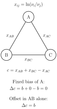
A loop tests consistency among comparisons. Changing the assigned frequency of A shifts both $x_{AB}$ and $x_{AC}$ by the same amount, so their contributions cancel. An error affecting only one comparison can produce nonzero closure. All three comparisons must be measured separately for the loop to provide an additional check.

What closure cannot tell you

Write $q_i=\ln(\nu_i/\nu_*)$ for an arbitrary common reference frequency $\nu_*$. Pairwise differences have the form $x_{ij}=q_i-q_j$. Any fixed bias that can be absorbed into one $q_i$ cancels around every loop. Thus a network can close perfectly even when each clock frequency has a fixed systematic error.

Nonzero closure can reveal inconsistencies specific to an individual link, comparison, or time interval. A time-dependent clock shift can also appear if the three comparisons sample different times. Zero closure therefore supports mutual consistency under the measurement model; it does not prove that all absolute frequencies are correct. Independent variation of fields, temperatures, trap conditions, and comparison methods provides additional physical tests. Beloy et al. (2021) give an experimental example of optical ratio comparisons through fibre and free-space links.

Gravitational redshift turns clocks into potential sensors

Clocks measure proper time along their trajectories. In a weak static gravitational field, using a coordinate time $t$ and Newtonian potential $\Phi$ that increases upward near Earth’s surface,

$$\frac{d\tau}{dt}\simeq 1+\frac{\Phi}{c^2}-\frac{v^2}{2c^2}.$$

For two clocks at rest in this coordinate system, the fractional rate difference is approximately $(\Phi_A-\Phi_B)/c^2$. The higher clock runs faster. Close to the surface, a small vertical separation $\Delta h$ gives

$$\frac{\Delta\nu}{\nu}\simeq\frac{g\Delta h}{c^2}.$$

The speed of light is denoted by $c$ in these relativistic equations; it is unrelated to the closure residual above. For real terrestrial comparisons, Earth’s rotation, tides, motion, and the definition of the reference potential must be treated consistently. An effective terrestrial potential can incorporate rotation rather than adding it twice.

A centimetre of height corresponds to a fractional rate difference of about $1.1\times10^{-18}$. Clocks actually compare gravitational potential, not geometric height alone: converting to height uses a gravity model. Bothwell et al. (2022) resolved a redshift gradient across different parts of one atomic sample. Such a differential measurement rejects some common noise; its uncertainty should not be read as the absolute systematic uncertainty of a complete clock.

Nuclear transitions require the same measurement discipline

The low-energy isomeric transition of $^{229}$Th lies in the vacuum ultraviolet, near $148$ nm. It can therefore connect nuclear structure to laser spectroscopy. Tiedau et al. (2024) demonstrated laser excitation in a solid host. Huang et al. (2026) reported a clock using feedback to synchronize a laser to a resolved thorium nuclear transition.

The nuclear origin of the transition changes its sensitivity to perturbations and to underlying constants. It does not eliminate the surrounding electronic and solid-state environment. In a crystal, local electric-field gradients, temperature, defects, and chemical environments can alter line positions or produce several distinguishable sites. Exciting a line, resolving its structure, locking an oscillator, and determining its corrected frequency answer different experimental questions.

To see the role of feedback, approximate the error signal near a selected line by

$$e_n=D(\nu_n-\nu_{\mathrm{res}})+\eta_n,\qquad \nu_{n+1}=\nu_n-Ge_n.$$

Here $D$ is the discriminator slope, $G$ the feedback gain, and $\eta_n$ the detection noise. For a fixed resonance and no additional delay, the detuning evolves as

$$\Delta_{n+1}=(1-GD)\Delta_n-G\eta_n.$$

The noiseless linear loop is stable when $0<GD<2$. It locks to the perturbed resonance $\nu_{\mathrm{res}}$; it does not infer the unperturbed nuclear frequency or remove the host shift. Real servos also have delays, drift, nonlinear capture ranges, and multiple noise sources. The simple model explains what locking accomplishes without treating it as a complete uncertainty analysis.

Clock comparisons can test changing constants

Suppose a dimensionless constant $\alpha$ changes slightly. For a chosen transition, a sensitivity coefficient relates the logarithmic frequency response to the perturbation. The measurable ratio response is

$$\delta\ln\frac{\nu_A}{\nu_B} =(K_{\alpha,A}-K_{\alpha,B})\frac{\delta\alpha}{\alpha} +\sum_j(K_{j,A}-K_{j,B})\frac{\delta X_j}{X_j}.$$

The $X_j$ are other dimensionless parameters in the specified theory. Sensitivity requires different responses: a perturbation that shifts both frequencies by the same fraction cancels. Environmental shifts must also be distinguished from the proposed signal. The transition sensitivities, the assumed field model, and the actual time sampling all enter a limit on new physics; see variation-of-constants searches.

A clock does not respond equally to all temporal frequencies. Ramsey interrogation averages the frequency difference over a finite window; dead time and asynchronous comparisons can introduce aliasing. Products of ordinary frequency-domain transfer functions are appropriate only for linear time-invariant stages. For pulsed or time-varying sampling, use the actual interrogation and comparison times. The Ramsey response plot shows why a larger static response can come with narrower bandwidth.

Exercises

1. Projection noise and cycle time

Take $\nu_0=4.29\times10^{14}$ Hz, $N=1000$, $T=1$ s, $C=0.8$, and $T_c=1.5$ s. Assume independent projection-noise-limited cycles. Find the single-cycle fractional uncertainty and the uncertainty after one hour. Express the long-time white-frequency-noise curve as $\sigma_y(\tau)=A/\sqrt{\tau/(1\,\mathrm{s})}$.

Solution

The single-cycle uncertainty is

$$u_{y,\mathrm{cycle}} =\frac{1}{2\pi(4.29\times10^{14})(1)(0.8)\sqrt{1000}} \simeq1.47\times10^{-17}.$$

One hour contains $3600/1.5=2400$ cycles, giving $u_y\simeq3.0\times10^{-19}$. The coefficient is $A=u_{y,\mathrm{cycle}}\sqrt{1.5}\simeq1.80\times10^{-17}$. Because one cycle lasts $1.5$ s, $A$ is a one-second normalization of the long-time white-noise curve, not an Allan deviation directly measured from one-second cycles. Additional correlated or systematic effects need not decrease as $\tau^{-1/2}$.

2. A consistent bias and an inconsistent comparison

Three separately measured log ratios have equal independent standard uncertainty $u$. Find the closure uncertainty. Then compare two changes: (a) the inferred log frequency of clock A increases by $b$ in both of its comparisons; (b) only the AB comparison increases by $b$.

Solution

Independence gives $u_c=\sqrt{3}u$. In (a), both $x_{AB}$ and $x_{AC}$ increase by $b$, so the closure changes by $b-b=0$. In (b), it changes by $b$. A closed loop cannot distinguish a fixed clock-frequency bias from a different true frequency. Correlated measurement errors require $u_c^2=\mathbf a^T\Sigma\mathbf a$ instead of $3u^2$.

3. Relativistic height sensitivity

Using $g=9.81\,\mathrm{m\,s^{-2}}$, convert a fractional rate difference of $10^{-18}$ to a local height difference. State the sign when clock A is above clock B and both are stationary under the stated approximation.

Solution

$$\Delta h=\frac{c^2}{g}10^{-18}\simeq9.2\times10^{-3}\ \mathrm m.$$

Clock A runs faster, so $(\nu_A-\nu_B)/\nu_B$ is positive for identical proper transition frequencies. This conversion assumes a locally constant $g$ and a consistently defined potential; a long-baseline comparison requires a fuller gravity and motion model.

4. Feedback follows a shifted line

In the linear nuclear-clock model, let $GD=1.2$ and ignore detection noise. How does an initial detuning evolve? If the host raises the resonance by a fixed $\delta\nu_{\mathrm{host}}$, does the loop remove that shift?

Solution

The detuning obeys $\Delta_n=(-0.2)^n\Delta_0$: it alternates in sign and shrinks. The loop converges to the shifted resonance. It therefore retains $\delta\nu_{\mathrm{host}}$ relative to the unperturbed transition; an independent estimate and correction are required. At $GD=2$ the noiseless error would alternate without shrinking, and for $GD>2$ this simple loop would be unstable.

References

• Beloy, K., et al. (Boulder Atomic Clock Optical Network Collaboration). “Frequency ratio measurements at 18-digit accuracy using an optical clock network.” Nature 591, 564–569 (2021). doi:10.1038/s41586-021-03253-4.
• Bothwell, T., Kennedy, C. J., Aeppli, A., Kedar, D., Robinson, J. M., Oelker, E., Staron, A., and Ye, J. “Resolving the gravitational redshift across a millimetre-scale atomic sample.” Nature 602, 420–424 (2022). doi:10.1038/s41586-021-04349-7.
• Huang, B., et al. “A nuclear clock synchronized to 229Th.” Nature (2026), published online 7 October 2026. doi:10.1038/s41586-026-11122-1.
• Ludlow, A. D., Boyd, M. M., Ye, J., Peik, E., and Schmidt, P. O. “Optical atomic clocks.” Reviews of Modern Physics 87, 637–701 (2015). doi:10.1103/RevModPhys.87.637.
• Tiedau, J., et al. “Laser excitation of the Th-229 nucleus.” Physical Review Letters 132, 182501 (2024). doi:10.1103/PhysRevLett.132.182501.