Cold Molecule Frontiers

Cold molecules combine controllable motion with rotational, vibrational, electronic, and nuclear-spin states. These extra states can provide strong interactions and sensitive measurements, but they also introduce decay, unwanted transitions, and state-dependent forces. Understanding both sides is essential when choosing a molecule for a particular experiment.

This page develops the physical comparisons behind molecular gases, arrays, and precision measurements. For dated demonstrations and open research questions, see Ultracold-molecule frontiers.

Required background. Cold molecules explains cooling, assembly, and trapping. Molecular quantum mechanics introduces the internal levels, and STIRAP explains coherent population transfer through a dark state.

Translational cooling and internal preparation are different

A low translational temperature means a narrow distribution of molecular velocities in the specified directions. It does not tell you how the molecules populate their rotational or vibrational levels. Conversely, an internally well-prepared sample can have appreciable motional excitation. An experiment therefore needs more than a temperature to describe its starting state.

Three examples make the distinction concrete:

• A slowed beam can have a low mean forward speed while retaining a broad velocity spread and several internal states. Mean speed and temperature are different quantities.
• A molecule assembled from two cold atoms can occupy a selected internal level while remaining excited in its trap.
• A molecular gas can be internally polarized without being quantum degenerate. Degeneracy depends on density and quantum statistics as well as temperature.

State population and purity also differ. The target-state population is $p_0=\langle0|\rho|0\rangle$, whereas the quantum purity is $\operatorname{Tr}\rho^2$. A pure superposition can have $p_0<1$. For a trapped particle, the motional ground-state population is a further quantity, measured by probes such as resolved sidebands rather than inferred solely from an internal-state measurement.

For a locally equilibrated dilute gas, the thermal wavelength $\lambda_T=h/\sqrt{2\pi m k_BT}$ gives the phase-space-density scale $n\lambda_T^3$. Its interpretation depends on geometry, interactions, and statistics. A Fermi gas is often characterized by $T/T_F$; a trapped Bose gas requires the appropriate condensation criterion. For a few particles outside equilibrium, a single fitted temperature may be an incomplete description.

Cooling and assembly start from different resources

Direct optical cooling removes momentum by repeated photon scattering. Molecular spontaneous emission can populate several vibrational and rotational levels, so additional lasers and state remixing may be needed to keep the molecule scattering. A diagonal Franck–Condon distribution helps with vibrational branching; it does not by itself close rotational, electronic, or hyperfine loss channels.

Assembly from ultracold atoms starts with atomic cooling and pairs atoms before transferring them into a selected molecular state. Association can produce a weakly bound molecule, followed by STIRAP into a deeply bound rovibrational level. This method avoids scattering many photons from the final molecule, but successful pair preparation and transfer must occur in the same trial. Ruttley et al. (2024) illustrate how assembly, state control, readout, and rearrangement can be combined in tweezers.

The elementary cooling and transfer derivations are in cold molecules and STIRAP. Here the useful comparison is what each method supplies for the next experiment: number of prepared molecules, internal population, motional distribution, lifetime, and repetition rate.

Preparation steps and site filling

Let the conditional probabilities of pair preparation, association, transfer, and survival be $p_{\rm pair}$, $p_{\rm assoc}$, $p_{\rm tr}$, and $p_{\rm surv}$. The probability of a molecule being available is

$$p_{\rm available} =p_{\rm pair}p_{\rm assoc}p_{\rm tr}p_{\rm surv}.$$

This product is the probability chain rule: the factors are conditioned on success of the preceding steps and need not represent independent processes. Detection efficiency adds another factor when counting detected molecules, but it does not change how many molecules were physically present. False-positive detections require an additional readout model.

Independence becomes a separate assumption when several sites are combined. If $M$ sites succeed independently with the same probability $p$, then $P_{\rm full}=p^M$. Common laser noise or a shared preparation failure can violate that assumption. A reservoir-and-rearrangement protocol changes the problem altogether: it uses the observed occupied sites instead of requiring every site to succeed on the first attempt.

Dipolar interactions depend on orientation and quantum state

A polar molecule has a molecule-frame electric dipole. A field-free rotational eigenstate of definite parity generally has zero mean dipole in the laboratory frame. An applied field can mix opposite-parity states and orient the molecule. Even when the mean dipole is zero, transition dipole matrix elements can still mediate resonant exchange.

For two fixed, parallel laboratory-frame dipoles of magnitude $d$, separated by $r$, the interaction reduces to

$$V_{\rm dd}(r,\theta)=\frac{d^2}{4\pi\epsilon_0r^3} \left(1-3\cos^2\theta\right),$$

where $\theta$ is the angle between the dipoles and the separation vector. Head-to-tail alignment is attractive; side-by-side alignment is repulsive. At $\theta=\arccos(1/\sqrt3)\simeq54.7^\circ$, this particular first-order interaction vanishes.

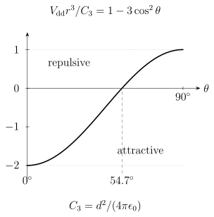
The sign of the interaction changes with geometry for fixed parallel dipoles. The zero at $54.7^\circ$ applies to this projected interaction; other state couplings, induced interactions, and higher-order terms need not vanish there. Rotational exchange uses transition matrix elements instead of simply substituting a permanent body-frame dipole.

The characteristic energy scale before angular and matrix-element factors is

$$\frac{d_{\rm eff}^2}{4\pi\epsilon_0hr^3} \simeq151\ {\rm Hz} \left(\frac{d_{\rm eff}}{1\ {\rm D}}\right)^2 \left(\frac{1\ \mu{\rm m}}{r}\right)^3.$$

Closer spacing strengthens interactions. It also amplifies fluctuations: for small longitudinal position changes, $\delta J/J\simeq-3\,\delta r/r$, provided the internal matrix elements and orientation remain fixed. Angular fluctuations can be particularly important near a zero of the angular factor, where a relative-error description fails. This is why motional cooling and trapping geometry enter a molecular gate, even if the chosen rotational states have long intrinsic lifetimes.

Exchange creates an entangled pair

In a resonant two-state subspace, choose phases so that the exchange matrix element $J$ is real:

$$H_{\rm ex}=J\left( |01\rangle\langle10|+|10\rangle\langle01| \right).$$

Ignoring all other shifts and couplings, an initial $|01\rangle$ evolves as

$$|\psi(t)\rangle= \cos(Jt/\hbar)|01\rangle-i\sin(Jt/\hbar)|10\rangle.$$

Equal populations at $t_B=\pi\hbar/(4|J|)$ give a maximally entangled state. At $t_S=2t_B$, the populations swap. With the common definition $\mathrm{iSWAP}|01\rangle=i|10\rangle$, positive $J$ produces the inverse iSWAP at $t_S$; local phase gates can convert it to iSWAP. Keeping the explicit state evolution avoids a sign ambiguity hidden in the gate name. Picard et al. (2025) demonstrate how dipolar exchange can be used for a molecular two-qubit gate.

For a large array, extending this model requires site-dependent couplings, detunings, and leakage channels. The lattice-model overview develops spin Hamiltonians; the molecular preparation and motion determine which terms are appropriate.

Elastic collisions and loss set different time scales

Evaporative cooling removes energetic particles and relies on collisions to redistribute energy among those that remain. A large elastic collision rate is helpful, but elastic collisions are not all equally effective at rethermalizing. Forward scattering changes direction and energy sharing only weakly; confinement and Pauli blocking can also affect relaxation.

For a tagged molecule, let $\Gamma_{\rm el}$ be its elastic-event rate and $\Gamma_{\rm loss}$ its removal-event rate in a specified stationary sample. In a simple model with constant competing Poisson rates,

$$\gamma=\frac{\Gamma_{\rm el}}{\Gamma_{\rm loss}},\qquad p_{\rm next,el}=\frac{\gamma}{1+\gamma}.$$

Rate coefficients quoted with different pair-counting or particle-loss conventions must be converted before being used in this expression. Neither this ratio nor a long lifetime alone determines the evaporation trajectory. Density, energy distributions, trap depth, one-body loss, three-body loss, and the rethermalization rate evolve during cooling.

Microwave shielding changes the approach to short range

Microwave fields mix rotational channels. In a suitable dressed state, approaching molecules can follow a repulsive potential that reduces their probability of reaching short separations, where reactive or inelastic loss occurs. Schindewolf et al. (2022) used microwave shielding to support evaporative cooling of polar molecules into a degenerate Fermi gas.

The shielding is a multichannel scattering process, not an impenetrable classical shell. Its effectiveness depends on detuning, coupling strength, polarization, collision energy, and nonadiabatic transitions. Increasing a microwave field can modify both elastic scattering and loss. Loss can also change because of density or background collisions, so comparing lifetimes without these quantities can be misleading.

The relevant calculations combine multichannel scattering with dressed molecular levels. An absorbing short-range boundary is a useful model of irreversible loss, but its assumed loss probability must be stated. Quantum statistics and the allowed partial waves matter before any field is applied.

Condensation, self-binding, and superfluidity are distinct

Different observables answer different many-body questions:

Physical property	What is being tested
Quantum degeneracy	Occupation statistics depart from a dilute classical gas; the relevant scales depend on statistics and confinement.
Bose condensation	An eigenvalue of the one-body density matrix becomes macroscopic in the appropriate limit. Momentum profiles and coherence measurements can support this interpretation.
Self-binding	The cloud remains localized without sufficient external confinement to bind it, over the observed time interval.
Density order	Spatial correlations show an ordered pattern, with finite-size and time dependence assessed.
Superfluid response	The system exhibits the appropriate phase stiffness, flow, rotational, or transport response.

A long-lived localized cloud need not be a condensate, and condensation alone does not establish superfluidity in every setting. Similarly, a modulated density image does not establish simultaneous density order and superfluid response. Molecular interactions offer ways to explore all of these questions, but a phase should be identified by the observables that define it. The current experimental comparisons are collected in ultracold-molecule research.

Precision measurements depend on detected information

Heavy molecules and opposite-parity doublets can give a strong response to symmetry-sensitive interactions. The molecule-internal effective field used in an electron-EDM analysis is a calculated response coefficient, not the externally applied electric field. Hutzler (2020) explains the opportunities offered by polyatomic structure.

For an ideal phase measurement with contrast $C$, $N_{\rm det}$ independent detected molecules, and interrogation time $T$, operation near the maximum fringe slope gives the statistical scale

$$u_{\Delta E}\simeq\frac{\hbar}{CT\sqrt{N_{\rm det}}}.$$

Cooling may increase $T$, but it can reduce the number available per unit time and introduce trap shifts. A fair comparison includes all these changes. Correlations or technical noise can invalidate the independent particle scaling.

A measured phase can depend on several effective interactions:

$$\phi=\frac{T}{\hbar} \left(K_e d_e+K_S C_S+\sum_jK_jg_j\right).$$

One measured combination does not generally give independent bounds on every coefficient. Fixing other coefficients to zero, placing prior constraints on them, or combining other measurements are different assumptions and lead to different conclusions. Precision molecular measurements develops the response coefficients and reversal methods.

Exercises

1: Assembly yield and array scaling

A molecular tweezer platform has independent end-to-end site success $p_{\rm mol}=0.48$ before rearrangement.

1. Find the probability of obtaining already full arrays with $M=8$ and $M=20$ sites.
2. How many independent 20-site attempts are required on average for one already full array?
3. Explain why this calculation does not predict the performance of a reservoir-and-rearrangement protocol.

Solution

For independent sites,

$$P_{\rm full}(M)=0.48^M.$$

Thus

$$\begin{aligned} P_{\rm full}(8) &=2.82\times10^{-3},\\ P_{\rm full}(20) &=4.22\times10^{-7}. \end{aligned}$$

The mean waiting count for independent Bernoulli attempts is

$$\langle n\rangle = \frac{1}{P_{\rm full}(20)} \simeq 2.37\times10^6.$$

The small probability motivates preparation protocols that use a reservoir. A reservoir-and-rearrangement protocol conditions on measured successes, moves molecules into target sites, and can repeat failed assembly. Its performance depends on reservoir size, imaging fidelity, move survival, correlated defects, and rebuild time. It is not described by $p_{\rm mol}^M$.

2: Competing elastic and loss events

For a tagged molecule, suppose the ratio of elastic-event to removal-event rates is $\gamma=460$. Treat the two processes as independent Poisson processes with constant rates, and classify each successive event as elastic or lossy.

1. What is the loss probability per event?
2. What is the probability of surviving 100 events?
3. Why is this not a complete evaporation model?

Solution

The per-event probabilities are

$$p_{\rm loss} = \frac{1}{1+\gamma} = \frac{1}{461} = 2.17\times10^{-3},$$

and

$$p_{\rm el} = \frac{460}{461}.$$

The simple survival probability is

$$P_{100} = \left(\frac{460}{461}\right)^{100} \simeq 0.805.$$

Real evaporation is not a fixed sequence of identical binary events. Density, temperature, trap depth, elastic cross section, one-body loss, three-body loss, and microwave dressing evolve. Evaporation also removes selected high-energy particles, so rethermalization and truncation efficiency must be modeled. The estimate is a simple comparison, not a prediction of final phase-space density.

3: Exchange phases and spacing

Take $d_{\rm eff}=1$ D and let the angular and state factors be one. At $r=2\,\mu{\rm m}$, find $J/h$, the Bell-state time, and the full swap time. For $J>0$, write the state at each time. How much larger is $J$ at $r=0.8\,\mu{\rm m}$ if the same model remains valid?

Solution

The scale is $J/h=151/2^3\simeq18.9$ Hz. Therefore

$$t_B=\frac{1}{8J/h}\simeq6.62\ {\rm ms},\qquad t_S=2t_B\simeq13.2\ {\rm ms}.$$

The states are $(|01\rangle-i|10\rangle)/\sqrt2$ and $-i|10\rangle$, respectively. On the full two-qubit space, with $|00\rangle$ and $|11\rangle$ unchanged by this model, the latter operation is inverse iSWAP. The interaction grows by $(2/0.8)^3=15.625$. This estimate neglects motion, other levels, and additional shifts; bringing traps closer can change those approximations.

4: Conditional fidelity with an explicit loss outcome

Each of two sites contains a molecule independently with probability $p=0.8$. In trials where both are present, the prepared state has target Bell-state overlap $F_{\rm pair}=0.94$. Assume failed trials are recorded as an orthogonal erasure state $|e\rangle$, and there are no false-positive pair detections. The cycle rate is $2\ {\rm s^{-1}}$.

Find the accepted-pair rate and the target-state overlap of the full output $\rho_{\rm out}=p^2\rho_{\rm pair}+(1-p^2)|e\rangle\langle e|$.

Solution

The pair probability is $0.64$, so the accepted rate is $1.28\ {\rm s^{-1}}$. Because the target Bell state is orthogonal to $|e\rangle$, its overlap with the full output is

$$\langle B|\rho_{\rm out}|B\rangle =p^2F_{\rm pair}=0.6016.$$

This is an unconditional state overlap for the explicitly defined output space. It is not a gate fidelity measured over all input states. A detected erasure can be handled differently from an undetected wrong qubit state. If failures can be misidentified as pairs, the simple conditional-state model must also include that readout error.

References

• Hutzler, N. R. “Polyatomic molecules as quantum sensors for fundamental physics.” Quantum Science and Technology 5, 044011 (2020). doi:10.1088/2058-9565/abb9c5.
• Picard, L. R. B., et al. “Entanglement and iSWAP gate between molecular qubits.” Nature 637, 821–826 (2025). doi:10.1038/s41586-024-08177-3.
• Ruttley, D. K., Guttridge, A., Hepworth, T. R., and Cornish, S. L. “Enhanced quantum control of individual ultracold molecules using optical tweezer arrays.” PRX Quantum 5, 020333 (2024). doi:10.1103/PRXQuantum.5.020333.
• Schindewolf, A., Bause, R., Chen, X.-Y., Duda, M., Karman, T., Bloch, I., and Luo, X.-Y. “Evaporation of microwave-shielded polar molecules to quantum degeneracy.” Nature 607, 677–681 (2022). doi:10.1038/s41586-022-04900-0.