Atom Interferometry

An atom interferometer coherently splits an atomic center-of-mass amplitude, lets the alternatives accumulate phase, and recombines them so that phase appears in measured populations or positions. The splitter can be a material grating, a standing optical wave, a two-photon Raman pulse, a Bragg pulse, a magnetic potential, or a guided-atom junction. The most widely used inertial configuration is the three-pulse light-pulse interferometer:

$$\frac{\pi}{2} \;-\; T \;-\; \pi \;-\; T \;-\; \frac{\pi}{2}.$$

The first pulse creates two momentum alternatives, the middle pulse redirects them, and the last pulse recombines them. For ideal instantaneous pulses and uniform acceleration,

$$\Phi_a = \mathbf k_{\mathrm{eff}} \mathbin{\cdot} \mathbf a\,T^2$$

in the convention used here. This compact formula is not the whole experiment. Its use requires a phase reference carried by the laser fields, controlled internal states, closed wave packets, known pulse timing, measured contrast, calibrated detection, and an account of vibration, rotation, wavefront, magnetic, optical, and gravity-gradient effects.

Atom interferometry is therefore both matter-wave physics and precision control. The atoms provide freely evolving quantum test masses; the light pulses provide beam splitters, mirrors, clocks, and rulers.

Required background. Interference with matter introduces matter-wave coherence; Ramsey interferometry supplies phase-sensitive pulse sequences; laser cooling supplies recoil and source preparation. Atom-interferometric sensors develops application-specific inference and systematic corrections.

Momentum Transfer and Laser Phase

Let a Raman process absorb from field 1 and stimulate emission into field 2. Define

$$\mathbf k_{\mathrm{eff}} = \mathbf k_1-\mathbf k_2,$$

and let a successful transition transfer momentum

$$\Delta\mathbf p = \hbar\mathbf k_{\mathrm{eff}}.$$

The effective optical phase is

$$\phi_L(\mathbf r,t) = \mathbf k_{\mathrm{eff}} \mathbin{\cdot} \mathbf r - \varphi(t),$$

where $\varphi(t)$ contains the microwave or optical frequency-difference phase synthesized by the laser system. A different sign convention for $\phi_L$ reverses several formulas together but cannot change a measured probability.

For the ideal three-pulse sequence, pulse centers occur at

$$t_1=0, \qquad t_2=T, \qquad t_3=2T.$$

The acceleration $\mathbf a$ means acceleration of the atoms relative to the optical phase fronts. Motion of a retroreflection mirror therefore enters the same observable as atomic acceleration, with the appropriate opposite relative sign.

The ideal output model is written

$$P_e = P_0 - \frac{C}{2} \cos \left( \Phi+\phi_{\mathrm{off}} \right),$$

where $P_0$ is an offset, $C$ is contrast, and $\phi_{\mathrm{off}}$ collects a controlled analysis phase and stable biases. An ideal balanced two-port interferometer has $P_0=1/2$ and $C=1$.

Matter Waves and Interferometer Phase

Center-of-mass phase

For a nonrelativistic center-of-mass path $\mathbf r(t)$ with Lagrangian $L$, the propagation amplitude carries phase

$$\phi_{\mathrm{prop}} = \frac{S}{\hbar}, \qquad S = \int L \left( \mathbf r,\dot{\mathbf r},t \right) dt.$$

Two alternatives can interfere only when the final measurement does not retain information that distinguishes them. Their propagation contribution is

$$\Delta\phi_{\mathrm{prop}} = \frac{S_u-S_\ell}{\hbar}.$$

This action language is universal, but a light-pulse atom interferometer also receives phases at each atom–light interaction. The observed phase is not generally just a classical action difference.

Propagation, laser, and internal phases

A useful decomposition is

$$\Phi = \Phi_{\mathrm{prop}} + \Phi_{\mathrm{laser}} + \Phi_{\mathrm{int}} + \Phi_{\mathrm{sep}}.$$

The terms are:

• $\Phi_{\mathrm{prop}}$: difference of center-of-mass actions along the arms;
• $\Phi_{\mathrm{laser}}$: optical phases imprinted at the pulses;
• $\Phi_{\mathrm{int}}$: phase from unequal internal-state dwell times and internal shifts;
• $\Phi_{\mathrm{sep}}$: phase associated with recombining wave packets that are not perfectly closed in position and momentum.

The decomposition can depend on gauge, frame, and phase convention, while the total $\Phi$ is observable. For quadratic external Hamiltonians and an ideal closed three-pulse geometry, large propagation and laser terms simplify to the familiar inertial phase.

External and internal paths

A Raman beam splitter correlates internal and external states:

$$|g,\mathbf p\rangle \longleftrightarrow |e,\mathbf p+\hbar\mathbf k_{\mathrm{eff}}\rangle.$$

The alternatives are therefore paths through both real space and internal Hilbert space. A Bragg process can transfer momentum while leaving the internal state unchanged. This distinction matters for magnetic sensitivity, differential light shifts, spontaneous scattering, and readout.

Source coherence

An ensemble need not be a Bose–Einstein condensate to interfere. Each atom can interfere with itself provided its wave packets are coherently split and recombined. Source temperature and size still matter because they set velocity spread, expansion, pulse efficiency, wavefront sampling, and ensemble dephasing.

Laser cooling and ultracold atoms explain source preparation. The interferometer begins with a characterized position, velocity, internal-state, and atom-number distribution.

Beam Splitters for Atoms

Architecture map

Method	Momentum mechanism	Internal state	Typical strengths	Typical limitations
material grating	diffraction at apertures or structures	unchanged	direct spatial atom optics	surface interactions, loss, fixed geometry
Raman–Nath or Kapitza–Dirac pulse	short standing-wave diffraction	usually unchanged	several diffraction orders, short interaction	multiport output, pulse-area sensitivity
Bragg diffraction	velocity-selective multiphoton diffraction	unchanged	clean momentum ports, large momentum transfer	narrow velocity acceptance, diffraction phase
stimulated Raman transition	two optical fields couple long-lived states	changed	internal-state labeling and state-selective readout	differential shifts, magnetic sensitivity
Bloch acceleration	adiabatic transport in an optical lattice band	unchanged or chosen	many photon recoils	lattice phase, adiabaticity, spontaneous scattering
magnetic or chip potential	state-dependent force or guide junction	often changed	compact guided geometries	roughness, interactions, trap noise

No beam splitter is described by a momentum label alone. Its unitary, velocity acceptance, internal-state action, spontaneous-emission probability, parasitic diffraction orders, and phase must all be calibrated.

Stimulated Raman transition

Consider two long-lived states $|g\rangle$ and $|e\rangle$ coupled through an optically excited manifold. For one-photon detuning $\Delta$ much larger than the excited-state linewidth and single-photon Rabi frequencies, the excited state can be approximately eliminated. A common effective coupling scale is

$$\Omega_{\mathrm{eff}} \simeq \frac{ \Omega_1\Omega_2^* }{ 2\Delta },$$

subject to polarization, Clebsch–Gordan coefficients, multiple excited levels, and convention-dependent factors.

The two-photon resonance condition contains internal, Doppler, and recoil terms:

$$\omega_1-\omega_2 = \omega_{eg} + \mathbf k_{\mathrm{eff}} \mathbin{\cdot} \mathbf v + \omega_{\mathrm{rec,eff}} + \delta_{\mathrm{LS}},$$

where

$$\omega_{\mathrm{rec,eff}} = \frac{ \hbar k_{\mathrm{eff}}^2 }{ 2m }$$

and $\delta_{\mathrm{LS}}$ represents differential light and other level shifts in the chosen sign convention.

For fixed optical phase across a resonant pulse, define its area

$$\theta = \int |\Omega_{\mathrm{eff}}(t)|\,dt,$$

one phase convention gives

$$|g,\mathbf p\rangle \longrightarrow{} \cos\frac{\theta}{2} |g,\mathbf p\rangle - i e^{i\phi_L} \sin\frac{\theta}{2} |e,\mathbf p+\hbar\mathbf k_{\mathrm{eff}}\rangle.$$

A $\pi/2$ pulse is a balanced splitter in the addressed two-state momentum subspace. A $\pi$ pulse swaps the two ports and acts as a mirror.

Counterpropagating geometry

For nearly counterpropagating fields of common wavelength $\lambda$,

$$k_{\mathrm{eff}} \simeq \frac{4\pi}{\lambda}.$$

The momentum separation is close to two single-photon recoils. Copropagating fields have much smaller $k_{\mathrm{eff}}$ and suppress inertial sensitivity; they are useful as diagnostics for internal-state shifts.

Reversing the momentum-transfer direction,

$$\mathbf k_{\mathrm{eff}} \longrightarrow -\mathbf k_{\mathrm{eff}},$$

reverses leading inertial phases. Some light shifts and magnetic phases do not reverse. Comparing the two directions is therefore a powerful discriminator, but imperfect reversal can leave residual bias.

Bragg diffraction

Bragg pulses couple momentum states within one internal level:

$$|g,\mathbf p\rangle \longleftrightarrow |g,\mathbf p+2n\hbar\mathbf k\rangle.$$

The integer $n$ is the Bragg order in an idealized two-beam geometry. Because the internal state is unchanged, Bragg interferometers can suppress some internal-state shifts. They still require control of velocity selection, optical phase, pulse shape, multiport diffraction, and drive-dependent diffraction phase.

Large momentum transfer

Additional Bragg, Raman, Bloch, or composite pulses can increase the arm separation to

$$\Delta p = N_\hbar\hbar k,$$

where $N_\hbar$ counts the net photon-recoil scale under a declared convention. A larger momentum separation held for the same duration increases spacetime area and inertial response. The complete pulse timing matters as well as maximum separation. It also magnifies wavefront errors, velocity selectivity, spontaneous scattering, pulse infidelity, and closure requirements.

Finite pulse duration

The instantaneous-pulse approximation requires pulse duration $\tau$ small compared with $T$ and with the timescale of the signal being measured. A finite pulse:

• samples acceleration during the interaction;
• changes the exact scale factor;
• gives velocity-dependent transfer;
• accumulates light shift and laser phase continuously;
• can populate parasitic momentum states; and
• modifies the sensitivity function near each pulse.

Precision work uses the actual envelope and effective Hamiltonian rather than replacing every pulse by an ideal matrix.

Three-Pulse Light-Pulse Interferometer

Pulse sequence

Start in $|g,\mathbf p\rangle$. In an ideal Raman sequence:

1. the first $\pi/2$ pulse creates amplitudes in $|g,\mathbf p\rangle$ and $|e,\mathbf p+\hbar\mathbf k_{\mathrm{eff}}\rangle$;
2. the $\pi$ pulse at $T$ exchanges the internal and momentum labels so the relative velocity reverses;
3. the last $\pi/2$ pulse at $2T$ mixes the alternatives; and
4. state-selective detection measures the two output ports.

In a frame following the mean trajectory, the two arms form a diamond in space–time.

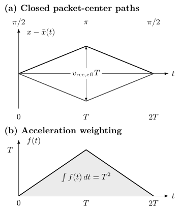
Top: relative packet centers separate by $v_{\mathrm{rec,eff}}T$ at the mirror pulse, then rejoin at $2T$. The last pulse mixes equal final momentum ports. Bottom: the acceleration weight has area $T^2$. For planar wavefronts the laser phase is $\phi_1-\phi_{2,u}-\phi_{2,\ell}+\phi_3$; the two middle phases equal twice the midpoint phase only under the appropriate spatial averaging.

Output probability

When pulse areas are ideal and unwanted ports are negligible, the two alternatives reaching one output add coherently. One output has

$$P_e = \frac12 \left[ 1-C\cos\Phi \right],$$

and the complementary output has $P_g=1-P_e$ if there is no loss or leakage. The minus sign follows the pulse convention below, for which three identical-axis pulses of total area $2\pi$ return the atom to $g$. Relabeling the port or shifting the analysis phase by $\pi$ changes the displayed fringe sign. The contrast $C$ can include imperfect overlap, ensemble averaging, and pulse errors as well as decoherence.

Laser-phase finite difference

For ideal instantaneous pulses, the imprinted phase has the structure

$$\Phi_{\mathrm{laser}} = \phi_1-2\phi_2+\phi_3,$$

where $\phi_2$ is the average of the two mirror-event phases: $\phi_2=(\phi_{2,u}+\phi_{2,\ell})/2$. The mirror acts on both arms in opposite transition directions. For planar wavefronts this average is the phase at the midpoint between their centers; for aberrated wavefronts it need not be.

If the phase fronts are planar and the effective optical phase is sampled along a reference trajectory $\mathbf r(t)$,

$$\begin{aligned} \Phi_{\mathrm{laser}} \supset{}& \mathbf k_{\mathrm{eff}} \mathbin{\cdot} \big[ \mathbf r(0) -2\mathbf r(T) +\mathbf r(2T) \big]. \end{aligned}$$

For

$$\mathbf r(t) = \mathbf r_0 + \mathbf v_0t + \frac12\mathbf a t^2,$$

the position and velocity terms cancel:

$$\mathbf r(0) -2\mathbf r(T) +\mathbf r(2T) = \mathbf aT^2.$$

After propagation and separation contributions are included, the closed uniform-acceleration result is

$$\Phi_a = \mathbf k_{\mathrm{eff}} \mathbin{\cdot} \mathbf aT^2.$$

Frequency chirp

A falling atom acquires a changing Doppler shift. The Raman frequency difference is commonly chirped so the pulses remain resonant. Let the synthesized phase contain

$$\varphi(t) = \varphi_0 + \omega_0t + \frac12\alpha t^2.$$

Then the quadratic phase contributes

$$-\alpha T^2$$

to the three-pulse finite difference. The leading phase becomes

$$\Phi = \left( \mathbf k_{\mathrm{eff}} \mathbin{\cdot} \mathbf a - \alpha \right) T^2 + \Phi_{\mathrm{sys}}.$$

Here $\alpha$ has angular-frequency chirp units, $\mathrm{rad\,s^{-2}}$. Scanning $\alpha$ finds the chirp that follows the atomic Doppler shift. The measurement is a comparison between atomic free fall and the laser phase fronts.

Rubidium recoil and gravity scales

For counterpropagating light near

$$\lambda = 780\ \mathrm{nm},$$

take

$$k_{\mathrm{eff}} \simeq \frac{4\pi}{\lambda} = 1.611\times10^7\ \mathrm{m^{-1}}.$$

For $^{87}\mathrm{Rb}$ with

$$m = 1.443\times10^{-25}\ \mathrm{kg},$$

the effective recoil velocity is

$$v_{\mathrm{rec,eff}} = \frac{\hbar k_{\mathrm{eff}}}{m} = 1.177\times10^{-2}\ \mathrm{m\,s^{-1}}.$$

At $T=0.100\ \mathrm s$, the maximum relative arm separation in the ideal sequence is approximately

$$\Delta x_{\max} = v_{\mathrm{rec,eff}}T = 1.18\ \mathrm{mm}.$$

The raw phase from standard gravity is large:

$$\begin{aligned} \Phi_g &= k_{\mathrm{eff}}gT^2 \\ &\simeq 1.58\times10^6\ \mathrm{rad}. \end{aligned}$$

The corresponding resonance-following chirp is

$$\frac{\alpha}{2\pi} = \frac{k_{\mathrm{eff}}g}{2\pi} \simeq 25.1\ \mathrm{MHz\,s^{-1}}.$$

Experiments do not usually count $1.58$ million radians from zero. They chirp near the expected value and estimate the residual phase, while tracking the integer-fringe and sign conventions.

Why no mass appears

The acceleration scale factor $k_{\mathrm{eff}}T^2$ contains no explicit atomic mass. The momentum kick is $\hbar k_{\mathrm{eff}}$, so the arm velocity separation is inversely proportional to mass, while the center-of-mass action is proportional to mass. These factors cancel in the ideal uniform-acceleration phase.

Mass still matters through recoil frequency, spatial separation, source expansion, diffraction resonance, interaction effects, and response to gradients. “Mass independent” applies to the leading scale factor, not to the complete apparatus.

Avoiding a phase-story trap

It is possible to rearrange the total phase among propagation, laser, and separation terms by changing coordinates or phase convention. Assigning the observed phase to only a gravitational potential term, only a proper-time term, or an enormous atomic “Compton clock” phase can be misleading unless the complete gauge- and frame-consistent interferometer is shown.

The invariant object is the measured phase difference predicted by the complete atom-plus-laser model.

Acceleration Response

Time-dependent acceleration

For ideal instantaneous pulses and an acceleration spatially uniform across both arms, define

$$f(t) = \begin{cases} t, & 0<t<T, \\ 2T-t, & T<t<2T, \\ 0, & \text{otherwise}. \end{cases}$$

The acceleration phase is

$$\Phi_a = \mathbf k_{\mathrm{eff}} \mathbin{\cdot} \int_0^{2T} f(t)\mathbf a(t)\,dt.$$

For constant acceleration,

$$\int_0^{2T} f(t)\,dt = T^2,$$

recovering $\Phi_a=\mathbf k_{\mathrm{eff}}\cdot\mathbf aT^2$.

The triangular weight shows that the interferometer does not measure instantaneous acceleration at one time. It measures a time-weighted combination over the complete sequence.

Mirror vibration

In a retroreflected geometry, displacement $z_m(t)$ of the reference mirror changes the effective laser phase. For ideal pulses,

$$\Phi_{\mathrm{vib}} \simeq -k_{\mathrm{eff}} \left[ z_m(0) -2z_m(T) +z_m(2T) \right]$$

when positive $z_m$ translates the effective phase fronts in the same direction as positive atomic position. This sign follows $\phi_L=k_{\mathrm{eff}}(z-z_m)-\varphi(t)$: only relative acceleration enters. The same contribution is $-k_{\mathrm{eff}}\int f(t)\ddot z_m(t)\,dt$.

Because $k_{\mathrm{eff}}$ is large, submicrometer mirror motion can sweep many fringes. Isolation, a classical accelerometer, feed-forward, correlation analysis, or common-mode differential interferometers are often essential.

Laser phase noise

A laser phase perturbation sampled by the pulses contributes

$$\delta\Phi_L = \delta\phi_L(0) -2\delta\phi_L(T) +\delta\phi_L(2T)$$

in the instantaneous limit. Finite pulses replace point samples by a sensitivity function. Oscillator phase noise, optical path noise, and phase lock noise must be filtered through that transfer function, not summarized only by an integrated linewidth.

Frequency response

For a sinusoidal acceleration, the triangular response has transform

$$F(\omega)=\int_0^{2T}f(t)e^{i\omega t}\,dt =T^2e^{i\omega T}\operatorname{sinc}^2\!\left(\frac{\omega T}{2}\right), \qquad \operatorname{sinc}x=\frac{\sin x}{x}.$$

It measures a weighted acceleration centered at $t=T$, with zeros at $\omega T=2\pi n$ for nonzero integers $n$. Finite pulses modify the response, especially at high frequencies; Cheinet et al. derive and measure this pulse-dependent sensitivity.

Rotation and the Matter-Wave Sagnac Phase

Coriolis form

In a frame rotating with angular velocity $\boldsymbol\Omega$, an atom with velocity $\mathbf v$ experiences Coriolis acceleration

$$\mathbf a_C = -2 \boldsymbol\Omega \mathbin{\times} \mathbf v.$$

Inserted into the acceleration scale factor, the leading rotation phase is

$$\begin{aligned} \Phi_\Omega &= -2T^2 \mathbf k_{\mathrm{eff}} \mathbin{\cdot} \left( \boldsymbol\Omega \mathbin{\times} \mathbf v \right) \\ &= 2T^2 \mathbf k_{\mathrm{eff}} \mathbin{\cdot} \left( \mathbf v \mathbin{\times} \boldsymbol\Omega \right). \end{aligned}$$

For constant $\boldsymbol\Omega$, the velocity here is the triangle-weighted mean trajectory velocity relative to the apparatus. If $\mathbf v(t)=\mathbf v_0+\mathbf a_0t$, it is $\mathbf v_0+\mathbf a_0T$. When $\mathbf a_0\parallel\mathbf k_{\mathrm{eff}}$, that acceleration term makes no Coriolis phase, leaving the transverse launch velocity. The expression is first order in rotation and assumes small trajectory deflections.

Enclosed-area form

For a matter-wave interferometer enclosing oriented area $\mathbf A$, the nonrelativistic Sagnac phase can be written

$$\Phi_\Omega = \frac{2m}{\hbar} \boldsymbol\Omega \mathbin{\cdot} \mathbf A.$$

In a light-pulse geometry,

$$\mathbf A = \frac{\hbar\mathbf k_{\mathrm{eff}}}{m} \mathbin{\times} \mathbf v\,T^2,$$

for constant transverse velocity and the oriented loop convention that gives the Coriolis sign above. More general trajectories require their actual oriented area.

Earth-rotation example

For maximum geometric projection, take

$$k_{\mathrm{eff}} = 1.611\times10^7\ \mathrm{m^{-1}}, \quad v = 0.50\ \mathrm{m\,s^{-1}}, \quad T = 0.100\ \mathrm s,$$

and

$$\Omega_\oplus = 7.292\times10^{-5}\ \mathrm{rad\,s^{-1}}.$$

Then

$$\begin{aligned} |\Phi_\Omega| &\simeq 2k_{\mathrm{eff}}v\Omega_\oplus T^2 \\ &= 11.7\ \mathrm{rad}. \end{aligned}$$

Earth rotation is therefore not automatically a tiny correction. It can be the signal in a gyroscope or a bias in a vertical accelerometer. Transverse velocity, beam direction, latitude, and mirror orientation must be measured.

Gravimetry, Gradiometry, and Inertial Sensing

Absolute gravimetry

A vertical interferometer compares atomic free fall with an optical phase reference tied to an instrument structure. The chirp rate that nulls the phase estimates the projection of gravitational acceleration along $\mathbf k_{\mathrm{eff}}$ after corrections:

$$\widehat g \simeq \frac{\widehat\alpha}{k_{\mathrm{eff}}} - \frac{\widehat\Phi_{\mathrm{sys}}}{ k_{\mathrm{eff}}T^2 }.$$

The reported value must specify sensor height, tides, atmospheric loading, polar motion, local mass distribution, vertical gravity gradient, and the instrument’s effective measurement height when those effects matter.

Differential gradiometry

Operate two interferometers at positions separated by baseline $\mathbf L$, interrogated by common laser pulses. Their phase difference is

$$\Delta\Phi \simeq \mathbf k_{\mathrm{eff}} \mathbin{\cdot} \left( \mathbf a_2-\mathbf a_1 \right) T^2.$$

For a slowly varying field,

$$\mathbf a_2-\mathbf a_1 \simeq \Gamma\mathbf L,$$

where $\Gamma$ is the gravity-gradient tensor. Common laser and mirror noise can cancel strongly, but unequal scale factors, timing, Rabi frequencies, wavefront sampling, and atom trajectories limit rejection.

Accelerometers and gyroscopes

An accelerometer maximizes $\mathbf k_{\mathrm{eff}}\cdot\mathbf a$. A gyroscope arranges nonzero transverse velocity or enclosed area so that $\boldsymbol\Omega\cdot\mathbf A$ is measurable. Multi-axis instruments use several beam directions, atomic trajectories, or simultaneous interferometers.

The same phase can contain both acceleration and rotation. Geometry, modulation, reversal, and auxiliary sensors are needed to separate them.

Recoil interferometers measure $h/m$ through a different phase combination; large-baseline force searches use still other time responses. Their sensitivities cannot be read directly from the simple gravimeter formula.

Wave-Packet Closure and Contrast

Closure in phase space

At recombination, corresponding wave packets should overlap in position, momentum, internal state, and all unobserved degrees of freedom. Let the residual displacement and momentum mismatch be

$$\Delta\mathbf x, \qquad \Delta\mathbf p.$$

For identical one-dimensional unchirped minimum-uncertainty Gaussian packets of rms width $\sigma_x$, displaced relative to each other, the overlap magnitude is

$$\left| \langle\psi_1|\psi_2\rangle \right| = \exp \left[ - \frac{\Delta x^2}{8\sigma_x^2} - \frac{\sigma_x^2\Delta p^2}{2\hbar^2} \right].$$

For a general common Gaussian state with covariance $\sigma_x^2,\sigma_p^2,\sigma_{xp}=\langle\{\delta x,\delta p\}\rangle/2$, the integrated contrast factor is instead

$$C_{\mathrm{overlap}} =\exp\!\left[-\frac{ \sigma_p^2\Delta x^2+\sigma_x^2\Delta p^2 -2\sigma_{xp}\Delta x\Delta p}{2\hbar^2}\right].$$

Free expansion produces a position–momentum correlation, so inserting the expanded width into the unchirped formula can be wrong. Roura, Zeller, and Schleich describe this phase-space geometry. An open interferometer can retain resolved spatial fringes while its integrated port contrast falls; this does not require irreversible environmental decoherence.

Averaging phases across the cloud

If atoms acquire phases $\delta\phi(\mathbf r,\mathbf v)$, the fringe amplitude is proportional to $\langle e^{i\delta\phi}\rangle$. Its modulus is the contrast factor and its argument is the phase bias. Neither is generally obtained by just inserting mean coordinates into the phase. Exercise 6 gives an exactly soluble wavefront-curvature example.

Which-path information

If an environment or uncontrolled internal degree of freedom ends in states $|E_u\rangle$ and $|E_\ell\rangle$ correlated with the two arms, the interference term is multiplied by

$$\langle E_\ell|E_u\rangle.$$

Spontaneous emission is especially destructive because the emitted photon can carry path, time, momentum, and internal-state information. Large one-photon detuning reduces excited-state population, but higher laser power may be required to preserve the two-photon Rabi rate.

Gravity gradients and open geometry

In a gravity gradient, trajectories do not close exactly under the pulse timing designed for uniform acceleration. Initial position and velocity can couple into the phase, and residual phase-space displacement can reduce contrast. Frequency shifts or modified mirror-pulse momentum transfer can help close the geometry, but the correction becomes part of the calibrated scale factor.

Detection and Phase Estimation

State-selective detection

Raman interferometers often detect the populations $N_g$ and $N_e$ by state-selective fluorescence, absorption imaging, or sequential shelving and repumping. A normalized output is

$$P_e = \frac{N_e}{ N_g+N_e },$$

after background, efficiency, and loss corrections justified by the detection model.

Normalization suppresses common atom-number fluctuations only if both state channels are linear and their relative calibration is stable.

Midfringe operation

The maximum probability slope occurs near quadrature:

$$\Phi+\phi_{\mathrm{off}} \simeq \frac{\pi}{2} \pmod{\pi}.$$

A controlled phase step on the last pulse can lock the interferometer near this point. If vibration noise spans many fringes, a nonlinear estimator can correlate atomic populations with an auxiliary accelerometer or with a second interferometer rather than linearizing one shot at a time.

Projection-noise baseline

For a balanced fringe with $P_0=1/2$, fixed contrast $C$, and $N$ independent Bernoulli detections at a fixed shot phase, the midfringe projection-noise scale is

$$\delta\Phi_{\mathrm{PN}} \simeq \frac{1}{ C\sqrt N }.$$

The corresponding acceleration uncertainty is

$$\delta a_{\mathrm{PN}} \simeq \frac{1}{ C\sqrt N\, k_{\mathrm{eff}}T^2 }.$$

For

$$N=10^6, \qquad C=0.50, \qquad T=0.100\ \mathrm s,$$

with the rubidium scale above,

$$\delta a_{\mathrm{PN}} \simeq 1.24\times10^{-8}\ \mathrm{m\,s^{-2}}$$

per shot. Detection noise, vibration, dead time, contrast fluctuations, wavefront effects, and drift commonly lie above this ideal baseline.

Sensitivity versus accuracy

Sensitivity describes statistical response or noise, often per shot or per square-root bandwidth. Accuracy concerns agreement with the defined measurand after systematic corrections. A highly sensitive interferometer can be inaccurate, and an accurate instrument can average slowly.

State the averaging time, cycle rate, bandwidth, estimator, rejection rules, and uncertainty model whenever a sensitivity or accuracy is quoted.

Geometry and Reversals

A fountain increases free-fall time but needs larger beams and control of rotation and gradients. Guided paths make a compact device but add path-dependent trapping phases. Delta-kick collimation narrows velocity spread; interactions or wavefront selection can still shift the fringe.

Reversing $\mathbf k_{\mathrm{eff}}$ changes both acceleration and leading Coriolis phase. Reversing transverse velocity changes the latter alone in the ideal model. Differential interferometers reject common mirror noise only to the extent that pulse timing and scale factors match. No reversal removes an effect with the same symmetry as the signal. Detailed estimators and uncertainty models are developed in atom-interferometric sensors.

Exercises

1. Raman recoil scales

For counterpropagating Raman beams at $\lambda=780\ \mathrm{nm}$ acting on $^{87}\mathrm{Rb}$ with mass

$$m=1.443\times10^{-25}\ \mathrm{kg},$$

calculate:

1. $k_{\mathrm{eff}}\simeq4\pi/\lambda$;
2. the effective recoil velocity $v_{\mathrm{rec,eff}}=\hbar k_{\mathrm{eff}}/m$; and
3. the effective recoil frequency $f_{\mathrm{rec,eff}}=\hbar^2k_{\mathrm{eff}}^2/(2mh)$.

Solution

The effective wave number is

$$\begin{aligned} k_{\mathrm{eff}} &= \frac{4\pi}{780\times10^{-9}\ \mathrm m} \\ &= 1.611\times10^7\ \mathrm{m^{-1}}. \end{aligned}$$

The recoil velocity is

$$\begin{aligned} v_{\mathrm{rec,eff}} &= \frac{ (1.0546\times10^{-34}) (1.611\times10^7) }{ 1.443\times10^{-25} } \\ &= 1.18\times10^{-2}\ \mathrm{m\,s^{-1}}. \end{aligned}$$

The kinetic recoil frequency is

$$\begin{aligned} f_{\mathrm{rec,eff}} &= \frac{ \hbar^2k_{\mathrm{eff}}^2 }{ 2mh } \\ &\simeq 1.51\times10^4\ \mathrm{Hz}. \end{aligned}$$

This is four times the single-photon recoil frequency because $k_{\mathrm{eff}}\simeq2k$ and recoil energy scales as wave number squared.

2. Fix the output-port sign

Use the resonant pulse matrix in the ordered basis $(g,e)$,

$$U(\theta,\phi)= \begin{pmatrix} \cos(\theta/2)&-ie^{-i\phi}\sin(\theta/2)\\ -ie^{i\phi}\sin(\theta/2)&\cos(\theta/2) \end{pmatrix}.$$

For a closed interferometer with propagation phases already included in the effective pulse phases, multiply the $\pi/2,\pi,\pi/2$ matrices. Find the excited-port probability.

Solution

Acting on $(1,0)^{\mathsf T}$ gives

$$a_e=\frac{i}{2}e^{i\phi_2} \left[e^{i(\phi_1-2\phi_2+\phi_3)}-1\right], \qquad P_e=\frac{1-\cos(\phi_1-2\phi_2+\phi_3)}2.$$

For equal phases the total rotation is $2\pi$ and $P_e=0$. A plus-sign fringe describes the complementary port or a $\pi$-shifted analysis phase, not the same unshifted convention.

3. Chirp-rate null

For vertical $k_{\mathrm{eff}}=1.611\times10^7\,\mathrm{m^{-1}}$ and $g=9.80665\,\mathrm{m\,s^{-2}}$, calculate the frequency chirp $\alpha/(2\pi)$ that nulls the leading gravity phase. If the applied chirp is larger by $100\ \mathrm{Hz\,s^{-1}}$, what residual phase appears at $T=0.100\ \mathrm s$?

Solution

The null condition is

$$\alpha = k_{\mathrm{eff}}g.$$

In ordinary-frequency chirp units,

$$\begin{aligned} \frac{\alpha}{2\pi} &= \frac{k_{\mathrm{eff}}g}{2\pi} \\ &= 25.1\ \mathrm{MHz\,s^{-1}}. \end{aligned}$$

An excess ordinary-frequency chirp of $100\ \mathrm{Hz\,s^{-1}}$ corresponds to angular chirp error

$$\delta\alpha = 2\pi(100)\ \mathrm{rad\,s^{-2}}.$$

The residual phase is

$$\delta\Phi = -\delta\alpha T^2 = -2\pi(100)(0.100)^2 = -2\pi\ \mathrm{rad}.$$

That is one complete fringe. The sign follows the chirp convention used in the page.

4. Use the triangular response

An extra constant acceleration $\delta a$ acts only during the first half of the sequence, $0<t<T$, and vanishes for $T<t<2T$. Find its phase contribution. Compare it with the phase from the same acceleration acting throughout the full sequence.

Solution

During the first interval, $f(t)=t$. Therefore

$$\begin{aligned} \delta\Phi_{\mathrm{first}} &= k_{\mathrm{eff}} \int_0^T t\,\delta a\,dt \\ &= \frac12 k_{\mathrm{eff}}\delta aT^2. \end{aligned}$$

If the same acceleration acts during the whole sequence,

$$\delta\Phi_{\mathrm{full}} = k_{\mathrm{eff}}\delta aT^2.$$

The first interval contributes half because the triangular response has equal area before and after the mirror pulse.

5. Earth-rotation phase

Assume the vectors are oriented for maximum projection and use

$$k_{\mathrm{eff}} = 1.611\times10^7\ \mathrm{m^{-1}}, \quad v=0.50\ \mathrm{m\,s^{-1}}, \quad T=0.100\ \mathrm s,$$

with

$$\Omega_\oplus = 7.292\times10^{-5}\ \mathrm{rad\,s^{-1}}.$$

Estimate the Coriolis rotation phase. What reversals help distinguish it from linear acceleration?

Solution

For maximum projection,

$$\begin{aligned} |\Phi_\Omega| &= 2k_{\mathrm{eff}}v\Omega_\oplus T^2 \\ &= 2 (1.611\times10^7) (0.50) (7.292\times10^{-5}) (0.100)^2 \\ &= 11.7\ \mathrm{rad}. \end{aligned}$$

Reversing transverse velocity reverses the rotation phase but not the leading acceleration phase. Reversing $\mathbf k_{\mathrm{eff}}$ reverses both. Combining momentum and velocity reversals, or comparing oppositely directed atomic trajectories, separates their reversal parities.

6. Curved wavefronts: phase bias and contrast together

Suppose every pulse has the same extra transverse phase $\phi_{\mathrm{wf}}=k_{\mathrm{eff}}r_\perp^2/(2R)$. Let atoms move ballistically transversely, with independent zero-mean Gaussian velocity components of variance $\sigma_v^2$. Calculate the ensemble fringe multiplier and its small-curvature acceleration bias.

Solution

The three-pulse finite difference cancels initial position:

$$\delta\Phi_{\mathrm{wf}} =\frac{k_{\mathrm{eff}}T^2}{R}(v_x^2+v_y^2) =b(v_x^2+v_y^2).$$

The two Gaussian integrals give

$$\left\langle e^{i\delta\Phi_{\mathrm{wf}}}\right\rangle =\frac{1}{1-2ib\sigma_v^2}.$$

Thus the contrast factor is $(1+4b^2\sigma_v^4)^{-1/2}$ and the phase bias is $\arctan(2b\sigma_v^2)$. Only when $|b|\sigma_v^2\ll1$ is the phase approximately its mean, $2b\sigma_v^2$, giving $\delta a\simeq2\sigma_v^2/R$. Changing source expansion can change both bias and visibility, even with perfect unitary dynamics. A varying curvature or velocity-selective detection requires a different average.

7. Wave-packet overlap

Two identical unchirped minimum-uncertainty Gaussian output packets have rms width $\sigma_x=50\ \mu\mathrm m$, residual displacement $\Delta x=20\ \mu\mathrm m$, and residual velocity mismatch $\Delta v=5.0\ \mu\mathrm{m\,s^{-1}}$ for $^{87}\mathrm{Rb}$. Estimate their overlap magnitude using

$$\left| \langle\psi_1|\psi_2\rangle \right| = \exp \left[ - \frac{\Delta x^2}{8\sigma_x^2} - \frac{\sigma_x^2m^2\Delta v^2}{2\hbar^2} \right].$$

Solution

The position-mismatch exponent is

$$\frac{\Delta x^2}{8\sigma_x^2} = \frac{(20)^2}{8(50)^2} = 0.020.$$

For

$$m=1.443\times10^{-25}\ \mathrm{kg},$$

the momentum-mismatch exponent is

$$\frac{\sigma_x^2m^2\Delta v^2}{2\hbar^2} \simeq 0.0585.$$

Thus

$$\left| \langle\psi_1|\psi_2\rangle \right| = \exp[-(0.020+0.0585)] \simeq 0.924.$$

Even a unitary interferometer can lose about $7.6\%$ of ideal amplitude visibility from this unresolved phase-space mismatch. An ensemble may lose more through averaging over packet parameters.

8. A chirped packet can retain overlap

Take $\hbar=1$, an initial pure Gaussian covariance $\sigma_x^2=\sigma_p^2=1/2$, $\sigma_{xp}=0$, and free expansion with $m=1$ for time $t=10$. For output mismatch $(\Delta x,\Delta p)=(1,0.1)$, compare the general covariance formula with the incorrect unchirped formula using only the expanded width.

Solution

Free evolution gives $\sigma_x^2=50.5$, $\sigma_p^2=0.5$, and $\sigma_{xp}=5$. The correct exponent is

$$\frac{0.5(1)^2+50.5(0.1)^2-2(5)(1)(0.1)}2=0.0025,$$

so $C=0.99750$. Backward free propagation maps the mismatch to $(\Delta x-t\Delta p,\Delta p)=(0,0.1)$, yielding the same answer. The width-only expression instead gives $1/(8\times50.5)+50.5(0.1)^2/2=0.25498$, or $C\simeq0.775$. It has discarded the position–momentum correlation.

References

• P. R. Berman, editor, Atom Interferometry, Academic Press (1997).
• C. J. Bordé, “Atomic interferometry with internal state labelling,” Physics Letters A 140, 10–12 (1989), doi:10.1016/0375-9601(89)90537-9.
• P. Cheinet, B. Canuel, F. Pereira Dos Santos, A. Gauguet, F. Yver-Leduc, and A. Landragin, “Measurement of the sensitivity function in a time-domain atomic interferometer,” IEEE Transactions on Instrumentation and Measurement 57, 1141–1148 (2008), doi:10.1109/TIM.2007.915148.
• A. D. Cronin, J. Schmiedmayer, and D. E. Pritchard, “Optics and interferometry with atoms and molecules,” Reviews of Modern Physics 81, 1051–1129 (2009), doi:10.1103/RevModPhys.81.1051.
• T. L. Gustavson, P. Bouyer, and M. A. Kasevich, “Precision rotation measurements with an atom interferometer gyroscope,” Physical Review Letters 78, 2046–2049 (1997), doi:10.1103/PhysRevLett.78.2046.
• M. Kasevich and S. Chu, “Atomic interferometry using stimulated Raman transitions,” Physical Review Letters 67, 181–184 (1991), doi:10.1103/PhysRevLett.67.181.
• M. Kasevich and S. Chu, “Measurement of the gravitational acceleration of an atom with a light-pulse atom interferometer,” Applied Physics B 54, 321–332 (1992), doi:10.1007/BF00325375.
• J. M. McGuirk, G. T. Foster, J. B. Fixler, M. J. Snadden, and M. A. Kasevich, “Sensitive absolute-gravity gradiometry using atom interferometry,” Physical Review A 65, 033608 (2002), doi:10.1103/PhysRevA.65.033608.
• A. Peters, K. Y. Chung, and S. Chu, “Measurement of gravitational acceleration by dropping atoms,” Nature 400, 849–852 (1999), doi:10.1038/23655.
• A. Roura, “Circumventing Heisenberg’s uncertainty principle in atom interferometry tests of the equivalence principle,” Physical Review Letters 118, 160401 (2017), doi:10.1103/PhysRevLett.118.160401.
• A. Roura, W. Zeller, and W. P. Schleich, “Overcoming loss of contrast in atom interferometry due to gravity gradients,” New Journal of Physics 16, 123012 (2014), doi:10.1088/1367-2630/16/12/123012.
• P. Storey and C. Cohen-Tannoudji, “The Feynman path integral approach to atomic interferometry: A tutorial,” Journal de Physique II 4, 1999–2027 (1994), doi:10.1051/jp2:1994103.