Quantum Wires

A quantum wire has discrete transverse modes and extended longitudinal motion. Each transverse state becomes a one-dimensional band, called a subband. Its band-edge density of states can be large even when its ideal conductance is finite: slowly moving electrons contribute many states per energy but carry proportionately less flux.

This page develops that connection through explicit state counting. It also explains when one subband has more than two Fermi points, why slowly varying confinement produces additional terms in a longitudinal model, and where interactions change the independent-electron picture. Quantum Point Contacts treats short constrictions, while Conductance Quantization develops terminal transmission and plateau measurements.

Required background. What Is Mesoscopic Physics? supplies the scale comparisons. Effective Mass supplies band-edge dispersion; Infinite Square Well supplies transverse boundary conditions. Fermi–Dirac Statistics supplies occupations.

Transverse confinement creates longitudinal subbands

Let the wire run along $x$. In a uniform separable effective-mass model with constant masses,

$$H=-\frac{\hbar^2}{2m_x}\partial_x^2+H_\perp.$$

The transverse Hamiltonian contains confinement in $y,z$. Solve

$$H_\perp\chi_n=\varepsilon_n\chi_n,$$

with normalized transverse modes. For periodic normalization length $L$,

$$\Psi_{nk}=L^{-1/2}e^{ikx}\chi_n,$$ $$E_n(k)=\varepsilon_n+\frac{\hbar^2k^2}{2m_x}.$$

The discrete label $n$ does not make the whole spectrum discrete: $k$ becomes continuous in a long wire. In this separable Hamiltonian the same longitudinal mass appears in every subband. Subband-dependent masses can arise from nonparabolicity or band mixing, but then they require an improved model rather than this separation alone.

Hard walls and smooth gates

For a rectangular hard-wall cross-section, put

$$\chi_{n_y n_z}(y,z)=u_{n_y}(y)u_{n_z}(z),$$ $$u_{n_j}(j)=\sqrt{\frac{2}{W_j}} \sin\!\left(\frac{n_j\pi j}{W_j}\right),$$

where $j=y,z$ and $n_j$ is a positive integer. The thresholds are

$$\varepsilon_{n_y n_z}=E_c+E_y n_y^2+E_z n_z^2,$$ $$E_j=\frac{\hbar^2\pi^2}{2m_jW_j^2}.$$

A split-gate channel in a two-dimensional electron gas already has vertical confinement. If only one vertical mode matters, the remaining lateral hard-wall thresholds are $\varepsilon_n=\varepsilon_z+E_1n^2$. For a harmonic lateral potential, they instead have equally spaced values $\varepsilon_z+\hbar\omega_y(n+1/2)$ with $n=0,1,\ldots$.

For the illustrative GaAs parameters $m^*=0.067m_e$ and lateral width $W=80\,\mathrm{nm}$,

$$\begin{aligned} E_1&\simeq0.877\,\mathrm{meV},\\ \varepsilon_2-\varepsilon_1&=3E_1\simeq2.63\,\mathrm{meV}. \end{aligned}$$

Finite barriers, depletion, electrostatic screening and band mixing change these numbers. The electronic width need not equal the fabricated width (Beenakker and van Houten).

Existence, occupation and resolution are separate

Confinement creates transverse modes even when an experiment cannot resolve their thresholds. A large cross-section can contain many closely spaced modes and admit a semiclassical approximation; the terminology should be accompanied by the occupied-mode count.

At zero temperature the lowest orbital mode alone is occupied when $\varepsilon_1<\mu<\varepsilon_2$. At finite temperature and bias, the occupied energy window also matters. Resolving neighboring thresholds requires thermal, instrumental and lifetime broadening to be small enough compared with their separation. Avoid counting the same escape or disorder contribution twice under different linewidth symbols.

None of these conditions ensures ballistic motion, phase coherence or a conductance plateau. Longitudinal metallic diffusion additionally requires an interval before localization; coherence depends on path duration and the environment. The mesoscopic scale lesson treats those independent comparisons.

Count occupied states and propagation directions

For a parabolic subband with $\mu>\varepsilon_n$,

$$k_{F,n}=\frac{\sqrt{2m_x(\mu-\varepsilon_n)}}{\hbar}.$$

Let $g_n$ count exactly degenerate internal states such as spin or valley, not propagation directions. The occupied interval is $-k_{F,n}<k<k_{F,n}$. Since the spacing of allowed $k$ values is $2\pi/L$, the zero-temperature line density is

$$n_{\rm 1D}=\sum_n\frac{g_n k_{F,n}}{\pi}.$$

Each ordinary parabola has two Fermi points, with opposite group velocities. The right-moving point supplies one incoming channel from the left reservoir, and the left-moving point supplies the opposite direction. Counting both as an additional factor in $g_n$ would double-count the states.

For a lateral hard-wall strip with fixed vertical mode, raising the chemical potential to the second threshold gives $k_{F,1}=\sqrt3\pi/W$. With spin degeneracy two, the density just before that opening is $2\sqrt3/W$, or $43.3\,\mu\mathrm m^{-1}$ for $W=80\,\mathrm{nm}$.

The one-dimensional density of states

For a general subband, define the density of states per unit length as $\rho_n(E)$. Every root of $E_n(k_i)=E$ contributes:

$$\rho_n(E)=\frac{g_n}{2\pi\hbar} \sum_i\frac{1}{|v_n(k_i)|},$$ $$v_n(k)=\frac{1}{\hbar}\frac{dE_n}{dk}.$$

For a parabola, the two roots have equal speed. Thus

$$\rho_n(E)=A_n\frac{\Theta(E-\varepsilon_n)}{\sqrt{E-\varepsilon_n}},$$ $$A_n=\frac{g_n}{\pi\hbar}\sqrt{\frac{m_x}{2}}.$$

The inverse-square-root singularity is a one-dimensional van Hove singularity. Many wave numbers fall within a small energy interval because the dispersion is flat near its minimum. The divergence is integrable:

$$\int_{\varepsilon_n}^{\varepsilon_n+\Delta E}\rho_n(E)dE =2A_n\sqrt{\Delta E}.$$

The number of states in a shrinking interval therefore tends to zero, not infinity.

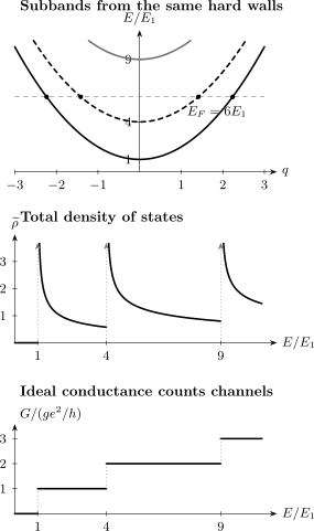
One model viewed three ways. With $q=kW/\pi$ and energy measured relative to the fixed vertical threshold, $E_n/E_1=n^2+q^2$. The middle panel shows $\widetilde\rho=2WE_1\rho/g$, summing all open subband contributions; its ideal singular peaks extend above the plotting range. The bottom panel counts perfectly transmitted modes. Density-of-states peaks and conductance steps occur at the same thresholds but have different shapes. A common internal degeneracy $g$ is factored out.

Finite temperature rounds the peak

For noninteracting electrons in a fixed confinement potential, the quantum capacitance per length is

$$c_q=e^2\frac{\partial n_{\rm 1D}}{\partial\mu},$$ $$\frac{c_q}{e^2}=\int dE\,\rho(E)K_T(E-\mu),$$

where $K_T=-\partial f/\partial E$. For one isolated parabolic threshold at $\mu=\varepsilon_n$, rescaling energy by $k_{\rm B}T$ gives

$$\frac{c_q}{e^2}=\frac{A_n}{\sqrt{k_{\rm B}T}}\,C,$$ $$C=\int_0^\infty\frac{x^{-1/2}\,dx}{4\cosh^2(x/2)} \simeq0.67372.$$

The finite-temperature value is finite and grows as $T^{-1/2}$ in this ideal model. This statement assumes a continuum of longitudinal states and negligible other broadening; finite length or lifetime eventually supplies another cutoff.

In a uniform single-gate electrostatic model, the measured electrochemical capacitance satisfies $c_\mu^{-1}=c_g^{-1}+c_q^{-1}$. With interactions, $c_q$ involves the thermodynamic compressibility, which need not equal the tunneling density of states and can even be negative while the total electrostatic system remains stable. Multiple gates, inhomogeneity and density-dependent confinement require the corresponding electrostatic treatment rather than a bare density-of-states fit.

Why a singular density of states gives a finite channel current

A right-moving branch contributes $g_n/(2\pi\hbar v_n)$ states per unit length per energy. Each state’s flux through a cross-section is proportional to $v_n$, so

$$v_n\rho_{n,+}(E)=\frac{g_n}{h}.$$

The low velocity and high state density cancel. With ideal reservoirs and elastic transmission,

$$G=\frac{e^2}{h}\sum_n g_n\mathcal T_n(\mu).$$

A perfectly transmitted spin-degenerate parabolic mode adds $2e^2/h$. If degeneracies are split or transmissions differ, count the actual resolved channels separately.

For an ideal step transmission $\mathcal T(E)=\Theta(E-\varepsilon_n)$, thermal averaging gives

$$G_n(T)=\frac{g_ne^2}{h} \frac{1}{1+e^{(\varepsilon_n-\mu)/(k_{\rm B}T)}}.$$

At the threshold it is half a step, while the thermally broadened capacitance has the $T^{-1/2}$ behavior above. This is a particularly direct way to distinguish flux from density. At the exact zero-temperature band edge, use the appropriate limiting prescription; the group velocity is zero there. The full terminal derivation and experimental qualifications are in Conductance Quantization.

An even subband can have more than two Fermi points

The two-point rule assumes a simple minimum and monotonic dispersion on either side. Spin–orbit coupling, hybridization or a more complicated band can produce several extrema. Count all energy roots and classify them by the sign of velocity, not the sign of $k$.

For a simple spin-resolved example, take

$$E(k)=E_0+E_b(q^2-1)^2,$$

where $q=k/k_0$ and $E_b>0$. Its minima are at $q=\pm1$, and the local maximum at $q=0$ has energy $E_0+E_b$. Put $e=(E-E_0)/E_b$. For $0<e<1$, four roots occur:

$$q=\pm\sqrt{1+\sqrt e},$$ $$q=\pm\sqrt{1-\sqrt e}.$$

Velocity has the sign of $q(q^2-1)$. The negative inner root and positive outer root move to the right. Above the central maximum, only the two outer roots remain. With ideal matched leads supporting these branches, the conductance therefore decreases from $2e^2/h$ to $e^2/h$ as energy passes that maximum. This is a change in the number of propagation branches, not negative transmission.

The general density-of-states formula still works. Below the central maximum, both inner and outer roots contribute; the inner pair gives an additional divergence as it merges at $q=0$. An even dispersion alone guarantees opposite partners, not exactly one pair. Real spin–orbit and multiband wires require their actual band Hamiltonian; see Spin–Orbit Coupling in Solids.

Slowly varying confinement and mode mixing

If the cross-section changes with $x$, local transverse states obey $H_\perp(x)\chi_n(x)=\varepsilon_n(x)\chi_n(x)$. Expanding the full state as $\Psi=\sum_n\phi_n(x)\chi_n(x)$ creates derivative couplings

$$P_{nm}=\langle\chi_n|\partial_x\chi_m\rangle_\perp,$$ $$Q_{nm}=\langle\chi_n|\partial_x^2\chi_m\rangle_\perp.$$

For constant longitudinal mass, define the differential operator

$$\mathcal K_{nm}=\delta_{nm}\partial_x^2 +2P_{nm}\partial_x+Q_{nm}.$$

The projected equations are

$$-\frac{\hbar^2}{2m_x}\sum_m\mathcal K_{nm}\phi_m =(E-\varepsilon_n)\phi_n.$$

Keeping only the local threshold and dropping every derivative of the basis is not the full projection. For an isolated mode, the diagonal adiabatic approximation contains a connection $\mathcal A_n$ and a nonnegative geometric potential $\Phi_n$:

$$H_n-V_n=\frac{(-i\hbar\partial_x-\mathcal A_n)^2}{2m_x},$$ $$V_n=\varepsilon_n+\Phi_n,$$ $$\mathcal A_n=i\hbar\langle\chi_n|\partial_x\chi_n\rangle,$$ $$\Phi_n=\frac{\hbar^2}{2m_x}\lVert\eta_n\rVert^2,$$ $$|\eta_n\rangle=(1-\Pi_n)|\partial_x\chi_n\rangle.$$

Here $\Pi_n=|\chi_n\rangle\langle\chi_n|$ projects onto the local transverse mode. Thus $\eta_n$ is the part of the mode’s spatial change orthogonal to the mode itself. Its squared norm makes the positive geometric contribution explicit. All these inner products integrate over the transverse coordinates. A change of transverse basis phase changes $\mathcal A_n$ and the longitudinal amplitude together, leaving predictions unchanged. Off-diagonal couplings must still be small for a single-mode approximation. A useful velocity-dependent test is $\hbar|v_xP_{nm}|\ll|\varepsilon_n-\varepsilon_m|$, supplemented by control of second-derivative terms and near-degeneracies.

Small mode conversion does not guarantee little reflection: an open channel also needs a sufficiently slowly varying longitudinal wave number, and a turning point can reflect even an uncoupled mode. Quantum Point Contacts develops the short-bottleneck limit.

Finite length, interactions and measurements

Reflections at both ends produce longitudinal resonances. Near a populated parabolic Fermi point, a hard-wall segment has spacing of order $\pi\hbar v_F/L$; near the band bottom use the discrete quadratic spectrum instead. Weak escape can resolve levels, but Coulomb charging additionally requires the appropriate capacitance and contact conditions. A visible Fabry–Pérot resonance is not automatically a Coulomb-blockaded dot. See Quantum Dots.

In a clean gapless interacting wire, low-energy density and spin excitations can form a Luttinger liquid (Haldane). Its tunneling exponents and collective velocities differ from the noninteracting subband-edge singularity. Carbon-nanotube power-law measurements and momentum-resolved tunneling experiments provide important examples, with their contact and energy-window assumptions (Bockrath and colleagues; Jompol and colleagues). Luttinger Liquid Preview develops the theory.

Strong internal correlations need not change the ideal two-terminal dc conductance in the same way as an isolated homogeneous model: clean wires connected appropriately to Fermi-liquid leads can have reservoir-controlled conductance (Maslov and Stone). This statement assumes the relevant clean, gapless transport limit; barriers, equilibration and gaps change the problem.

Probe	Quantity to connect to the model
Gate and bias spectroscopy	Thresholds, transmission, degeneracy and gate lever arm
Capacitance	Compressibility plus geometric electrostatics
Momentum-resolved tunneling	Spectral dispersion and possible collective velocities
Optical transitions	Electron–hole levels, excitons and selection rules
Magnetic-field response	Spin splitting and orbital changes to confinement

Do not assume an in-plane field has negligible orbital coupling in a finite-thickness or cylindrical wire. Compare orientation and transverse length scales with the magnetic length. Likewise, topological edge channels have their own boundary mechanism; one-dimensional propagation does not make them ordinary confinement subbands.

Exercises

1. Width, energy and occupation

For a lateral hard-wall channel with $m^*=0.067m_e$ and $W=60\,\mathrm{nm}$, find $E_1$, the spacing to the second mode, and the spin-degenerate line density just before that mode opens. Use $\hbar^2/(2m_e)=38.10\,\mathrm{meV\,nm^2}$.

Solution

The hard-wall expression gives $E_1\simeq1.56\,\mathrm{meV}$. The spacing is $3E_1\simeq4.68\,\mathrm{meV}$, and the threshold line density is $2\sqrt3/W\simeq57.7\,\mu\mathrm m^{-1}$.

These use a fixed vertical mode, hard walls and a parabolic band. A gate-dependent smooth potential does not generally preserve the same spacing or density formula.

2. A peak and a step at the same energy

For one isolated parabolic subband at $\mu=\varepsilon_n$, derive the thermal scaling of $c_q$ by substituting $E-\varepsilon_n=k_{\rm B}Tx$. Compare with its ideal conductance at that chemical potential.

Solution

The factors $dE$, $(E-\varepsilon_n)^{-1/2}$ and $K_T$ give net factor $(k_{\rm B}T)^{-1/2}$. Thus

$$\frac{c_q}{e^2}=\frac{0.67372A_n}{\sqrt{k_{\rm B}T}}.$$

The dimensionless integral is finite because $x^{-1/2}$ is integrable at zero and the Fermi weight decays exponentially at infinity. The conductance is $g_ne^2/(2h)$ for the ideal thermally averaged step. It does not share the capacitance’s divergent low-temperature scale. Other levels, finite length and broadening must remain negligible for this comparison.

3. Four roots, two right movers

For $E=E_0+E_b(q^2-1)^2$, find the Fermi roots at $e=1/4$ and $e=9/4$, classify their velocities and count ideal right-moving channels.

Solution

At $e=1/4$ the roots are $\pm\sqrt{3/2}$ and $\pm1/\sqrt2$. The derivative is proportional to $q(q^2-1)$, so $+\sqrt{3/2}$ and $-1/\sqrt2$ move right: two incoming channels.

At $e=9/4$, only $\pm\sqrt{5/2}$ are real roots, giving one right mover. The negative inner root in the first case is a useful reminder that momentum sign and velocity sign need not agree.

4. The geometric potential of a changing Gaussian mode

Let a normalized real transverse ground state be

$$\chi(y;x)=\frac{e^{-y^2/[2a(x)^2]}}{\pi^{1/4}\sqrt{a(x)}}.$$

Show that its connection vanishes and compute $\Phi$ using $\langle y^2\rangle=a^2/2$ and $\langle y^4\rangle=3a^4/4$.

Solution

Differentiating gives

$$\partial_x\chi=\frac{a'}{a} \left(\frac{y^2}{a^2}-\frac12\right)\chi.$$

Its overlap with $\chi$ vanishes, so $\mathcal A=0$. The squared norm is $\langle\partial_x\chi|\partial_x\chi\rangle=(a'/a)^2/2$. Hence

$$\Phi=\frac{\hbar^2}{4m_x}\left(\frac{a'}{a}\right)^2.$$

The positive term survives in the diagonal adiabatic model even though the real mode has no Berry connection. It does not remove the need to check couplings to excited transverse modes.

5. Discrete levels near and far from the band bottom

An isolated segment has hard walls at $x=0,L$ and fixed transverse energy $\varepsilon$. Compute the exact longitudinal level spacing and compare with $\pi\hbar v/L$ at a large quantum number $j$.

Solution

The levels are $E_j=\varepsilon+Aj^2$, where $A=\hbar^2\pi^2/(2m_xL^2)$ and $j=1,2,\ldots$. Therefore

$$E_{j+1}-E_j=A(2j+1).$$

At $k_j=j\pi/L$, the linearized estimate is $\pi\hbar v_j/L=2Aj$. Its relative error is $1/(2j+1)$ compared with the exact spacing, small only at large $j$. Opening the contacts broadens these levels; observing charge blockade requires additional charging physics.

References

• C. W. J. Beenakker and H. van Houten, “Quantum Transport in Semiconductor Nanostructures,” Solid State Physics 44, 1–228 (1991), doi:10.1016/S0081-1947(08)60091-0.
• M. Bockrath et al., “Luttinger-Liquid Behaviour in Carbon Nanotubes,” Nature 397, 598–601 (1999), doi:10.1038/17569.
• F. D. M. Haldane, “‘Luttinger Liquid Theory’ of One-Dimensional Quantum Fluids. I. Properties of the Luttinger Model and Their Extension to the General 1D Interacting Spinless Fermi Gas,” Journal of Physics C: Solid State Physics 14, 2585–2609 (1981), doi:10.1088/0022-3719/14/19/010.
• Y. Jompol et al., “Probing Spin–Charge Separation in a Tomonaga–Luttinger Liquid,” Science 325, 597–601 (2009), doi:10.1126/science.1171769.
• D. L. Maslov and M. Stone, “Landauer Conductance of Luttinger Liquids with Leads,” Physical Review B 52, R5539–R5542 (1995), doi:10.1103/PhysRevB.52.R5539.

Further reading

• S. Datta, Electronic Transport in Mesoscopic Systems, Cambridge University Press (1995), doi:10.1017/CBO9780511805776.
• T. Giamarchi, Quantum Physics in One Dimension, Oxford University Press (2004), doi:10.1093/acprof:oso/9780198525004.001.0001.