Hall Effect

The Hall effect is the antisymmetric part of linear electrical response: a current driven along one axis produces a transverse electric field. A magnetic field or magnetic order can select the orientation of that response. In its simplest form, the Lorentz force deflects mobile charge until a transverse electrostatic field balances that deflection. In real quantum matter, the same measurement can also contain multiple carrier types, anisotropic scattering, Berry-curvature velocity, magnetic order, real-space spin texture, or a quantized two-dimensional response.

That variety makes the Hall effect unusually informative and unusually easy to overinterpret. A Hall slope can determine carrier density only within a validated one-carrier model. A positive slope need not prove that every Fermi-surface pocket is hole-like. A zero-field transverse signal need not scale with net magnetization. A plateau is not merely an ordinary Hall line with an especially precise slope.

The theory below connects signed Hall tensors to ordinary carriers, multiple bands, Berry curvature and scattering. Hall measurements explains how terminal voltages and magnetic sweep histories are converted into these coefficients. Drude theory supplies the relaxation-time model and Boltzmann transport its collision equation.

Helpful background. Conventions fixes charge and tensor signs, Drude Theory supplies the one-carrier benchmark, and Boltzmann Transport with Fermi Surface supports the multiband semiclassical branch. Berry Curvature supports the intrinsic anomalous-Hall branch.

Charge, field and Hall-voltage conventions

Hall signs are meaningful only after the axes, tensor order, charge convention, and voltage polarity are fixed. Throughout this page:

• $(x,y,z)$ is a right-handed coordinate system;
• the imposed longitudinal current has $j_x>0$;
• the magnetic induction is $\mathbf B=B_z\hat{\mathbf z}$;
• $q$ is signed, with $q=-e$ for electrons and $q=+e$ for holes;
• the Hall resistivity is

$$\rho_{yx} \equiv \left. \frac{E_y}{j_x} \right|_{j_y=0};$$

• the weak-field Hall coefficient is

$$R_{\mathrm H} \equiv \lim_{B_z\to0} \frac{\rho_{yx}(B_z)}{B_z}.$$

The in-plane conductivity tensor for an isotropic or fourfold-symmetric system is written

$$\begin{pmatrix} j_x\\ j_y \end{pmatrix} = \begin{pmatrix} \sigma_{xx} & \sigma_{xy}\\ -\sigma_{xy} & \sigma_{xx} \end{pmatrix} \begin{pmatrix} E_x\\ E_y \end{pmatrix}.$$

Its inverse is

$$\begin{pmatrix} E_x\\ E_y \end{pmatrix} = \frac{1}{ \sigma_{xx}^2+\sigma_{xy}^2 } \begin{pmatrix} \sigma_{xx} & -\sigma_{xy}\\ \sigma_{xy} & \sigma_{xx} \end{pmatrix} \begin{pmatrix} j_x\\ j_y \end{pmatrix}.$$

Therefore

$$\rho_{xx} = \frac{\sigma_{xx}}{ \sigma_{xx}^2+\sigma_{xy}^2 }, \qquad \rho_{yx} = \frac{\sigma_{xy}}{ \sigma_{xx}^2+\sigma_{xy}^2 }.$$

Some literature instead names $E_x/j_y$ as $\rho_{xy}$, or writes the antisymmetric conductivity entries in the opposite order. Those are legitimate conventions, but formulas cannot be transferred between them by inspection. The explicit tensor above fixes every sign below.

Hall-Bar Geometry and Measured Voltage

Consider a rectangular bar of width $w$ along $y$, thickness $t$ along $z$, and current $I_x$ along $x$. In a uniform three-dimensional sample,

$$j_x = \frac{I_x}{wt}.$$

For top and bottom contacts separated along $+y$, define $V_{\mathrm H}=\phi_{\mathrm{bottom}}-\phi_{\mathrm{top}}=E_yw$ in a uniform field. Then

$$\rho_{yx} = \frac{V_{\mathrm H}t}{I_x}.$$

An actual voltmeter measures a scalar-potential difference. Because $\mathbf E=-\boldsymbol\nabla\phi$, the lead polarity must be mapped explicitly onto the stated definition of $V_{\mathrm H}$. Swapping the leads reverses the reported sign without changing the sample.

For a two-dimensional conducting sheet, thickness is not part of the response:

$$R_{yx}^{\square} = \frac{V_{\mathrm H}}{I_x}.$$

The three-dimensional $\rho_{yx}$ has units of $\Omega\,\mathrm m$, whereas the sheet Hall resistance has units of $\Omega$. Likewise, $R_{\mathrm H}$ has units of $\mathrm{m^3/C}$ for a bulk density and $\mathrm{m^2/C}$ for a sheet density.

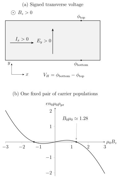
The sign convention fixes $j_x>0$, $B_z>0$, and $\rho_{yx}=E_y/j_x$. A one-carrier hole response has positive slope and an electron response negative slope. The solid curve is a schematic two-band response whose low- and high-field signs differ; Hall sign is therefore not a literal count of pocket types.

Classical One-Carrier Hall Effect

Take carriers of density $n$, signed charge $q$, isotropic mass $m^*$, and transport time $\tau$. Their steady drift velocity obeys

$$0 = q\left( \mathbf E+\mathbf v_d\times\mathbf B \right) - \frac{m^*\mathbf v_d}{\tau}.$$

With $\mathbf B=B_z\hat{\mathbf z}$, the component equations are

$$\begin{aligned} \frac{m^*}{\tau}v_x &= q(E_x+B_zv_y), \\ \frac{m^*}{\tau}v_y &= q(E_y-B_zv_x). \end{aligned}$$

Under open-circuit conditions $j_y=0$, one carrier species has $v_y=0$. The transverse equation immediately gives

$$E_y=v_xB_z,\qquad j_x=nqv_x,\qquad \rho_{yx}=\frac{B_z}{nq}.$$

Thus $R_{\mathrm H}=1/(nq)$: electrons have a negative slope and holes a positive slope in this convention. The collision time cancels because it controls the drift needed for a given longitudinal field, while the transverse field balances the Lorentz force at the measured current. Drude theory derives the full field-dependent conductivity and its exact inversion, including $\rho_{xx}=m^*/(nq^2\tau)$.

What the minimal result does and does not say

The same model predicts no longitudinal magnetoresistance:

$$\rho_{xx}(B_z)=\rho_{xx}(0).$$

This cancellation is special to one isotropic parabolic band with one constant $\tau$. A measured field dependence of $\rho_{xx}$ is not a failure of tensor algebra; it is evidence that at least one simplifying assumption is inadequate.

The Hall angle in this convention is

$$\tan\theta_{\mathrm H} \equiv \frac{\rho_{yx}}{\rho_{xx}} = \frac{\sigma_{xy}}{\sigma_{xx}} = \frac{qB_z\tau}{m^*}.$$

Only when $|\tan\theta_{\mathrm H}|\ll1$ may one use

$$\rho_{yx} \simeq \frac{\sigma_{xy}}{\sigma_{xx}^2}.$$

Replacing resistivity by conductivity without checking this condition can corrupt both magnitudes and scaling exponents.

Hall Coefficient, Density, and Mobility

In the one-carrier model,

$$n = \frac{1}{|qR_{\mathrm H}|}, \qquad \mu_{\mathrm H} \equiv |R_{\mathrm H}|\sigma_{xx}(0) = \mu.$$

These reductions require one relevant carrier species of known charge in a uniform conducting volume or sheet, with approximately isotropic parabolic transport, no important parallel channel and a Hall factor near one. Their field range must match the weak-field definition. They are not definitions of the physical carrier density or drift mobility.

In a doped semiconductor, $1/(e|R_{\mathrm H}|)$ is often called the Hall density. The name should preserve the qualification: it need not equal a chemical dopant density, a total band filling, or a quantum-oscillation carrier count.

Energy-dependent scattering and the Hall factor

Even one isotropic nondegenerate parabolic band in three spatial dimensions can depart from $R_{\mathrm H}=1/(nq)$ when $\tau$ depends on energy. Assuming a finite positive first lifetime moment and a finite second moment, the standard weak-field treatment gives

$$R_{\mathrm H} = \frac{r_{\mathrm H}}{nq}, \qquad r_{\mathrm H} = \frac{ \left\langle\tau^2\right\rangle }{ \left\langle\tau\right\rangle^2 }.$$

For this result, the average is weighted by the current-carrying states:

$$\left\langle X\right\rangle = \frac{ \displaystyle \int_0^\infty d\epsilon\, \epsilon^{3/2} \left( -\frac{\partial f_0}{\partial\epsilon} \right) X(\epsilon) }{ \displaystyle \int_0^\infty d\epsilon\, \epsilon^{3/2} \left( -\frac{\partial f_0}{\partial\epsilon} \right) }.$$

If $\tau(\epsilon)\propto\epsilon^r$ down to the band edge in the nondegenerate limit, require $r>-5/4$ for the second moment to converge; this also ensures convergence of the first moment. Then

$$r_{\mathrm H} = \frac{ \Gamma\!\left(\frac52+2r\right) \Gamma\!\left(\frac52\right) }{ \Gamma^2\!\left(\frac52+r\right) }.$$

The gamma-function expression represents these convergent integrals; analytic continuation outside their domain does not define a physical Hall factor. Cauchy–Schwarz implies $r_{\mathrm H}\ge1$ for this positive weighting. In a strongly degenerate metal with a smooth $\tau(\epsilon)$, the thermal window narrows around the Fermi energy and $r_{\mathrm H}\to1$. Band anisotropy and anisotropic scattering require more general tensor factors; they cannot always be compressed into one universal scalar $r_{\mathrm H}$.

Multiband Hall Transport

Suppose independent carrier groups $a$ have density $n_a$, signed charge $q_a$, and positive mobility $\mu_a$. For isotropic bands their Drude conductivities add:

$$\sigma_{xx}(B_z) = \sum_a \frac{ n_a|q_a|\mu_a }{ 1+\mu_a^2B_z^2 },$$ $$\sigma_{xy}(B_z) = \sum_a \frac{ n_aq_a\mu_a^2B_z }{ 1+\mu_a^2B_z^2 }.$$

The measured resistivities follow only after the summed tensor is inverted. At weak field,

$$R_{\mathrm H} = \frac{ \displaystyle \sum_a n_aq_a\mu_a^2 }{ \displaystyle \left( \sum_a n_a|q_a|\mu_a \right)^2 }.$$

The numerator weights mobility quadratically. A small population of highly mobile carriers can therefore set the Hall sign even when another population dominates the number of states.

Electron–hole model

For electron density $n$, hole density $p$, and mobilities $\mu_e,\mu_h>0$,

$$R_{\mathrm H}(0) = \frac{ p\mu_h^2-n\mu_e^2 }{ e\left( p\mu_h+n\mu_e \right)^2 }.$$

The exact two-carrier Hall resistivity is

$$\rho_{yx}(B_z) = \frac{B_z}{e} \frac{ p\mu_h^2-n\mu_e^2 +(p-n)\mu_e^2\mu_h^2B_z^2 }{ \left(p\mu_h+n\mu_e\right)^2 +(p-n)^2\mu_e^2\mu_h^2B_z^2 }.$$

At fixed nonzero charge imbalance $p-n$, the asymptotic $|B_z|\to\infty$ limit is

$$\rho_{yx}(B_z) \longrightarrow \frac{B_z}{e(p-n)}.$$

The high-field approximation is controlled when the $B_z^2$ terms in both numerator and denominator of the full fraction dominate their respective constant terms. For the denominator this condition is

$$|p-n|\mu_e\mu_h|B_z| \gg p\mu_h+n\mu_e.$$

Near compensation this field can greatly exceed both individual mobility fields. Thus $|\mu_eB_z|,|\mu_hB_z|\gg1$ alone is not a sufficient finite-field test; use the full fraction and the compensation crossover rather than assigning an asymptote prematurely.

The weak-field sign is mobility weighted; the high-field sign approaches the net charge imbalance. A sign reversal between these limits is therefore possible without any field-induced change of band topology.

At compensation, $p=n$, the nominal high-field expression is singular and the full formula must be retained. More generally, the limit assumes closed semiclassical orbits, field-independent densities and mobilities, and no magnetic breakdown. Open Fermi surfaces, density-wave reconstruction, quantum oscillations, or field-driven phase changes can invalidate it.

Identifiability of a multiband fit

A nonlinear $\rho_{yx}(B)$ is compatible with multiple bands, but different densities and mobilities can fit the same restricted field interval. Simultaneous $\rho_{xx}$ and $\rho_{yx}$ data constrain the same summed conductivity tensor more tightly than either alone. Gate capacitance, stoichiometry, spectroscopy and quantum oscillations can then constrain density independently. A fitted mobility also predicts where $\mu B$ becomes appreciable; if no such crossover is resolved, its numerical value may be weakly determined. Hall measurements develops the fitting and uncertainty analysis.

Fermi-Surface and Boltzmann View

The scalar formula $R_{\mathrm H}=1/(nq)$ conceals the geometry of a crystal band. In weak magnetic field, the Lorentz term moves a wave packet along a constant-energy surface:

$$\hbar\dot{\mathbf k} = q\mathbf v_n(\mathbf k)\times\mathbf B.$$

Within a relaxation-time treatment, the first magnetic correction to the conductivity can be written

$$\sigma_{ij}^{(1)} = - \frac{q^3}{\hbar} \sum_n \int_{\mathrm{BZ}} \frac{d^dk}{(2\pi)^d} \left( -\frac{\partial f_0}{\partial\epsilon} \right) \tau_n v_{n,i} \qquad\qquad \times \left( \mathbf v_n\times\mathbf B \right) \cdot \boldsymbol\nabla_{\mathbf k} \left( \tau_n v_{n,j} \right).$$

For an isotropic parabolic band and constant $\tau$, this reduces to the Drude result. For an anisotropic Fermi surface, the curvature of the velocity field and the variation of the mean free path matter. Consequently:

• a single connected band can have a nontrivial Hall coefficient;
• electron-like and hole-like regions can coexist on a complicated Fermi surface;
• scattering anisotropy can change the Hall response without changing the enclosed volume;
• an interacting metal need not admit a simple carrier-density interpretation.

At stronger field, carriers retain memory around longer portions of their semiclassical orbit. The Chambers formula on Boltzmann Transport provides the corresponding velocity-history construction.

Transverse voltage and field parity

An imperfect contact alignment mixes longitudinal and transverse voltages. Taking the odd part $[R_{yx}^{\mathrm{raw}}(B)-R_{yx}^{\mathrm{raw}}(-B)]/2$ removes an even pickup only when the two measurements represent the appropriate paired states. In a hysteretic magnet, opposite fields on the same sweep are generally not time-reversed states; opposite branches may be paired only when their magnetic history has the needed symmetry. Exchange bias or a fixed magnetic component can spoil that pairing.

Nor is every even transverse voltage a contact error: anisotropic resistivity produces the planar Hall signal described below. A general four-terminal longitudinal resistance need not be even in field; reciprocity exchanges current and voltage leads as well as reversing time-reversal-odd state variables. Hall measurements treats polarity, branch pairing and geometry explicitly. The result must be converted to a resistivity tensor before inversion; the small-Hall-angle shortcut is not valid near a quantized plateau or for a large anomalous signal.

Ordinary and Anomalous Hall Effects

The ordinary Hall effect is the field-odd orbital response associated with the Lorentz force and the carrier dynamics described above. In a magnetic material, an additional transverse response can track magnetic order even as the external field tends to zero. A useful phenomenological decomposition is

$$\rho_{yx}(B,M) = R_0B + \rho_{yx}^{\mathrm A}(M).$$

Here $R_0B$ denotes the ordinary contribution and $\rho_{yx}^{\mathrm A}$ the anomalous Hall contribution. Writing the decomposition this way avoids silently mixing magnetic induction $B$ with magnetic field $H$ or absorbing convention-dependent factors of $\mu_0$ into an anomalous coefficient.

The formula is a fitting organization, not a microscopic derivation. It is most credible when magnetization independently saturates, the high-field ordinary slope is reproducible, and the decomposition works across temperature, orientation, and sweep history. In a multiband magnet, the ordinary term need not be linear in field, so a constant $R_0$ is already an approximation. In a metamagnet, the band structure and scattering can change with $M$. A straight-line subtraction is then not guaranteed to isolate a unique anomalous signal.

Intrinsic Berry-Curvature Contribution

For a nondegenerate Bloch band, adopt the Berry connection and curvature

$$\mathbf A_n(\mathbf k) = i \left\langle u_{n\mathbf k} \middle| \boldsymbol\nabla_{\mathbf k} u_{n\mathbf k} \right\rangle,$$ $$\boldsymbol\Omega_n(\mathbf k) = \boldsymbol\nabla_{\mathbf k} \times \mathbf A_n(\mathbf k).$$

The wave-packet velocity contains an anomalous term:

$$\dot{\mathbf r} = \frac{1}{\hbar} \boldsymbol\nabla_{\mathbf k} \widetilde\epsilon_n - \dot{\mathbf k} \times \boldsymbol\Omega_n.$$

At zero external magnetic field, $\hbar\dot{\mathbf k}=q\mathbf E$, so the anomalous velocity is transverse to $\mathbf E$. The resulting intrinsic Hall conductivity in the convention of this page is

$$\sigma_{xy}^{\mathrm{int}} = - \frac{q^2}{\hbar} \sum_n \int_{\mathrm{BZ}} \frac{d^dk}{(2\pi)^d} f_n(\mathbf k) \Omega_{n,z}(\mathbf k).$$

This is an occupied-state property of the band wavefunctions. It does not require a Lorentz-force deflection or an asymmetric impurity collision. Near avoided crossings opened by spin–orbit coupling, Berry curvature can become strongly concentrated and make the intrinsic anomalous Hall response sensitive to chemical potential.

Symmetry constraints

Time reversal relates Berry curvature at opposite crystal momenta:

$$\boldsymbol\Omega_n(\mathbf k) \xrightarrow{\mathcal T} - \boldsymbol\Omega_{\bar n}(-\mathbf k).$$

In thermal equilibrium with unbroken time reversal, paired states have equal occupations and the linear charge Hall conductivity vanishes. Inversion instead makes Berry curvature even in momentum. When both symmetries hold, the Abelian curvature of an isolated nondegenerate band vanishes pointwise wherever that description is valid.

Broken time reversal is necessary for an equilibrium linear anomalous charge Hall effect, but a large uniform magnetization is not. Noncollinear antiferromagnets can have nearly zero net moment and still possess a symmetry-allowed Berry-curvature integral. The magnetic space group, not merely the scalar $M$, decides whether $\sigma_{xy}$ is allowed.

Filled two-dimensional bands

For a completely filled isolated two-dimensional band,

$$C_n = \frac{1}{2\pi} \int_{\mathrm{BZ}} d^2k\, \Omega_{n,z}(\mathbf k) \in\mathbb Z.$$

The intrinsic formula becomes

$$\sigma_{xy} = - C\frac{e^2}{h}, \qquad C=\sum_{n\in\mathrm{filled}}C_n.$$

This is the geometric bridge between anomalous Hall response in bands and quantized Hall conductance. The sign follows the Berry-curvature and tensor conventions stated above; changing either convention changes the displayed sign but not the measured physics.

Extrinsic Anomalous Hall Mechanisms

Disorder and scattering also generate anomalous Hall response. The traditional mechanism labels are useful, but in a multiband spin–orbit-coupled material their separation can depend on the theoretical representation.

Skew scattering

Write $W(\mathbf k'\leftarrow\mathbf k)$ for the transition rate from incoming $\mathbf k$ to outgoing $\mathbf k'$. Skew scattering has a nonzero part antisymmetric under interchange of these channels:

$$W_{\mathrm A}(\mathbf k'\leftarrow\mathbf k) =\frac12\left[ W(\mathbf k'\leftarrow\mathbf k) -W(\mathbf k\leftarrow\mathbf k') \right].$$

For a magnetic state, an allowed term proportional to $\mathbf M\cdot(\mathbf k\times\mathbf k')$ changes sign under this interchange while remaining even under simultaneous momentum inversion $(\mathbf k,\mathbf k')\mapsto(-\mathbf k,-\mathbf k')$. Thus skew scattering does not require inversion breaking. Nagaosa and collaborators (2010) distinguish this rate asymmetry from time-reversal reciprocity, which also reverses the magnetic state. The asymmetric collision term produces a transverse component of the nonequilibrium distribution. In the conventional clean-limit regime,

$$\sigma_{xy}^{\mathrm{skew}}\propto\tau, \qquad \sigma_{xx}\propto\tau.$$

At small Hall angle this implies

$$\rho_{yx}^{\mathrm{skew}} \propto \rho_{xx}.$$

Side jump

During a spin–orbit-coupled scattering event, a wave packet can acquire a coordinate shift transverse to its incoming direction. The event rate scales as $\tau^{-1}$ while the nonequilibrium occupation scales as $\tau$, leaving the conventional side-jump conductivity of order $\tau^0$. Its resistivity contribution therefore often scales as

$$\rho_{yx}^{\mathrm{sj}} \propto \rho_{xx}^2$$

at small Hall angle.

The intrinsic Berry-curvature conductivity is also of order $\tau^0$ in the clean metallic regime. This motivates the empirical scaling form

$$\rho_{yx}^{\mathrm A} = a\rho_{xx} + b\rho_{xx}^2.$$

The linear term is often associated with skew scattering and the quadratic term with intrinsic plus side-jump response. That association is a diagnostic, not a proof. Temperature can change phonon and impurity scattering differently, longitudinal channels can mix, and the intrinsic Berry-curvature integral can itself change with magnetization or chemical potential. A mechanism claim should combine scaling with microscopic calculation, controlled disorder variation, and symmetry information.

Distinguishing Other Transverse Responses

Several effects can resemble an anomalous Hall trace:

Effect	Essential ingredient	Key distinction
Planar Hall effect	Anisotropic magnetoresistance with in-plane field or order	Commonly even under reversal of the axial field and depends on in-plane angle
Topological Hall contribution	Real-space spin chirality and adiabatic coupling	Extracted residual is model dependent; subtraction alone does not establish a skyrmion phase
Spin Hall effect	Transverse spin current from spin–orbit coupling	Charge Hall voltage may vanish under time reversal
Thermal Hall effect	Transverse heat transport	Requires thermal-gradient and heat-current definitions, including magnetization-current corrections
Nonlinear Hall effect	Second- or higher-order electric response	Can occur in a time-reversal-invariant but inversion-broken metal; scales nonlinearly with drive

For example, an in-plane unit magnetic direction $\mathbf m=(\cos\varphi,\sin\varphi)$ and anisotropic resistivity $\rho_{ij}=\rho_\perp\delta_{ij}+\Delta\rho\,m_im_j$ give $\rho_{yx}=\rho_{xy}=\Delta\rho\sin\varphi\cos\varphi$. This transverse voltage is symmetric in its tensor indices and unchanged by $\mathbf m\to-\mathbf m$. Its conventional name, planar Hall effect, does not make it an antisymmetric Hall conductivity.

The phrase “topological Hall effect” is especially vulnerable to overclaiming. A hump left after subtracting fitted ordinary and anomalous backgrounds is not by itself a real-space topology measurement. Imaging, scattering, field-angle dependence, and a controlled model of the magnetic texture are needed.

Quantum Hall Bridge

In a sufficiently clean two-dimensional electron system at strong perpendicular field, the Hall response ceases to be a smooth semiclassical line. Landau quantization reorganizes the spectrum, and the integer quantum Hall regime exhibits plateaus

$$|\sigma_{xy}| = N\frac{e^2}{h}, \qquad \sigma_{xx}\simeq0.$$

When $\sigma_{xx}\to0$,

$$\rho_{yx} = \frac{1}{\sigma_{xy}}, \qquad \rho_{xx}\to0.$$

Here $N$ is the positive integer labeling a Hall plateau. The filling factor instead measures the carrier density relative to the Landau-level degeneracy:

$$\nu = \frac{n_{2\mathrm D}h}{e|B_z|}$$

for a simple two-dimensional gas, with $n_{2\mathrm D}$ including all spin and valley populations. Resolved or unresolved degeneracies determine which integer plateaus occur; they do not add a second factor to this density formula. In the clean integer-filled limit, $\nu=N$. Across a disorder-broadened plateau, localized bulk states can fill while $\nu$ changes and $N$ stays fixed; see filling and the plateau integer. Integer plateaus arise when the chemical potential lies in a mobility gap: bulk states at the Fermi level are localized while chiral edge transport remains. The robustness is tied to an integer Chern number, not to an exceptionally accurate estimate of a Drude relaxation time.

The ordinary and quantum Hall effects are connected but not interchangeable:

• the ordinary result follows from semiclassical force balance and depends continuously on density;
• the integer quantum Hall value is a two-dimensional conductance fixed by $e^2/h$ and a topological integer;
• disorder is detrimental to mobility yet helps broaden plateaus by localizing bulk states;
• edge channels and bulk topology supply a description absent from the one-carrier Drude model.

Landau Levels derives the orbital spectrum, Chern Numbers explains the topological invariant, and Quantum Hall Discovery records the experimental milestone. Integer Quantum Hall Effect develops plateau formation, edge states, localization, flux insertion, and resistance metrology.

Exercises

1. A signed voltage and a tensor correction

A uniform film has thickness $t=100\,\mathrm{nm}$ and current $I_x=1\,\mathrm{mA}$. Its top-minus-bottom potential is $+2\,\mathrm{mV}$ and its longitudinal resistivity is $\rho_{xx}=10^{-6}\,\Omega\,\mathrm m$. Find $\rho_{yx}$ and $\sigma_{xy}$. By what fraction would the approximation $\rho_{yx}/\rho_{xx}^2$ overestimate the magnitude?

Solution

Our signed Hall voltage is bottom-minus-top, so $V_{\mathrm H}=-2\,\mathrm{mV}$ and

$$\begin{aligned} \rho_{yx}&=V_{\mathrm H}t/I_x=-2\times10^{-7}\,\Omega\,\mathrm m,\\ \sigma_{xy}&=\frac{\rho_{yx}}{\rho_{xx}^2+\rho_{yx}^2} \simeq-1.923\times10^5\,\mathrm{S/m}. \end{aligned}$$

The shortcut gives $-2.0\times10^5\,\mathrm{S/m}$. Its magnitude exceeds the exact result by the factor $1+(\rho_{yx}/\rho_{xx})^2=1.04$, a 4% error. Lead polarity and tensor inversion are separate steps; correcting one does not correct the other.

2. A two-band sign reversal

Use dimensionless parameters $p=1$, $n=1.4$, $\mu_h=2$, and $\mu_e=1$. Determine the weak-field sign, the high-field sign, and the nonzero field at which the exact two-band $\rho_{yx}$ changes sign.

Solution

The weak-field numerator is

$$p\mu_h^2-n\mu_e^2 = 4-1.4 = 2.6>0,$$

so the initial Hall slope is hole-like. At high field, $p-n=-0.4<0$, so $\rho_{yx}\to B/[e(p-n)]$ is electron-like.

The nonzero crossing satisfies

$$p\mu_h^2-n\mu_e^2 + (p-n)\mu_e^2\mu_h^2B_0^2 = 0.$$

Thus

$$B_0^2 = \frac{2.6}{1.6}, \qquad B_0 \simeq 1.28$$

in the reciprocal-mobility field units used for the parameters. No carrier density changes at the crossing.

3. Bound on the Hall factor

Prove $r_{\mathrm H}\ge1$ for the positive transport weighting used in the one-band Hall factor, assuming $0<\langle\tau\rangle<\infty$ and $\langle\tau^2\rangle<\infty$. When does equality hold?

Solution

Normalize the positive weight so that $\langle1\rangle=1$. Cauchy–Schwarz applied to $\tau$ and $1$ gives

$$\langle\tau\rangle^2 \le \langle\tau^2\rangle \langle1\rangle = \langle\tau^2\rangle.$$

Therefore

$$r_{\mathrm H} = \frac{\langle\tau^2\rangle}{\langle\tau\rangle^2} \ge1.$$

Equality holds when $\tau$ is constant over all states carrying nonzero weight.

4. Scaling is not mechanism identification

In the small-Hall-angle regime, show why $\sigma_{xy}^{\mathrm{skew}}\propto\tau$ gives $\rho_{yx}^{\mathrm A}\propto\rho_{xx}$, whereas a $\tau^0$ Hall conductivity gives $\rho_{yx}^{\mathrm A}\propto\rho_{xx}^2$. Explain why observing these powers is not a unique microscopic diagnosis.

Solution

For small Hall angle,

$$\rho_{yx}^{\mathrm A} \simeq \frac{\sigma_{xy}^{\mathrm A}}{\sigma_{xx}^2}, \qquad \rho_{xx} \simeq \frac{1}{\sigma_{xx}}.$$

Since $\sigma_{xx}\propto\tau$, a skew term $\sigma_{xy}^{\mathrm{skew}}\propto\tau$ gives $\rho_{yx}^{\mathrm{skew}}\propto\tau^{-1}\propto\rho_{xx}$. A $\tau^0$ intrinsic or side-jump term gives $\rho_{yx}\propto\tau^{-2}\propto\rho_{xx}^2$.

The inference is not unique because several scattering channels can have different temperature dependence, intrinsic Berry curvature can change with magnetic order or chemical potential, side-jump and intrinsic terms share the same leading power, and the approximation fails at large Hall angle.

References

• N. W. Ashcroft and N. D. Mermin, Solid State Physics (Holt, Rinehart and Winston, 1976), Chapters 12 and 13.
• L. Berger, “Side-Jump Mechanism for the Hall Effect of Ferromagnets,” Physical Review B 2, 4559–4566 (1970), doi:10.1103/PhysRevB.2.4559.
• R. G. Chambers, “The kinetic formulation of conduction problems,” Proceedings of the Physical Society. Section A 65, 458–459 (1952), doi:10.1088/0370-1298/65/6/114.
• F. D. M. Haldane, “Berry Curvature on the Fermi Surface: Anomalous Hall Effect as a Topological Fermi-Liquid Property,” Physical Review Letters 93, 206602 (2004), doi:10.1103/PhysRevLett.93.206602.
• E. H. Hall, “On a New Action of the Magnet on Electric Currents,” American Journal of Mathematics 2, 287–292 (1879), doi:10.2307/2369245.
• R. Karplus and J. M. Luttinger, “Hall Effect in Ferromagnetics,” Physical Review 95, 1154–1160 (1954), doi:10.1103/PhysRev.95.1154.
• N. Nagaosa, J. Sinova, S. Onoda, A. H. MacDonald, and N. P. Ong, “Anomalous Hall effect,” Reviews of Modern Physics 82, 1539–1592 (2010), doi:10.1103/RevModPhys.82.1539.
• N. A. Sinitsyn, “Semiclassical theories of the anomalous Hall effect,” Journal of Physics: Condensed Matter 20, 023201 (2008), doi:10.1088/0953-8984/20/02/023201.
• D. J. Thouless, M. Kohmoto, M. P. Nightingale, and M. den Nijs, “Quantized Hall Conductance in a Two-Dimensional Periodic Potential,” Physical Review Letters 49, 405–408 (1982), doi:10.1103/PhysRevLett.49.405.
• K. von Klitzing, G. Dorda, and M. Pepper, “New Method for High-Accuracy Determination of the Fine-Structure Constant Based on Quantized Hall Resistance,” Physical Review Letters 45, 494–497 (1980), doi:10.1103/PhysRevLett.45.494.
• D. Xiao, M.-C. Chang, and Q. Niu, “Berry phase effects on electronic properties,” Reviews of Modern Physics 82, 1959–2007 (2010), doi:10.1103/RevModPhys.82.1959.
• J. M. Ziman, Principles of the Theory of Solids, 2nd ed. (Cambridge University Press, 1972), Chapters 7 and 9.