Thermoelectric Response

Thermoelectric response couples electrical flow to heat flow. A temperature gradient can drive charge, and an electrical current can carry heat even at uniform temperature. The measured coefficients depend on which current or gradient is constrained. In particular, the thermal conductivity of an electrically open sample is a Schur complement of the coupled response matrix:

$$\boldsymbol\kappa =\bar{\boldsymbol\kappa} -T\widetilde{\boldsymbol\alpha} \boldsymbol\sigma^{-1}\boldsymbol\alpha.$$

The subtraction describes the heat carried by the compensating electrochemical field. Omitting it can misidentify both electronic heat conduction and thermoelectric efficiency. This page develops the material coefficients and their interpretation in drag, bipolar and transverse effects. Transport Coefficients explains the general current–force relations; Boltzmann Transport derives the kinetic approximation.

Required background. Transport Coefficients Preview supplies constitutive coefficients, transport limits and reciprocity.

Helpful background. Boltzmann Transport supplies energy moments for quasiparticles; Kubo Formula in Materials supplies microscopic response and current definitions; Phonons supplies lattice heat carriers; Transport Measurements supplies voltage and geometry conventions.

Charge, heat and electrochemical driving

Consider local dc linear response near equilibrium at temperature $T>0$. Use SI bulk current densities: charge current $\mathbf j$ in $\mathrm{A/m^2}$ and heat current $\mathbf j_Q$ in $\mathrm{W/m^2}$. A sheet or finite device needs its corresponding normalization and boundary problem.

For a single charged species, let $q$ be its signed charge, $\mu$ its chemical potential and $\phi$ the electric potential. The electrochemical force per unit charge is

$$\begin{aligned} \boldsymbol{\mathcal E} &=\mathbf E-\frac{\boldsymbol\nabla\mu}{q} =-\boldsymbol\nabla V_{\mathrm{ec}},\\ V_{\mathrm{ec}}&=\phi+\frac{\mu}{q}, \qquad \mathbf E=-\boldsymbol\nabla\phi. \end{aligned}$$

For electrons, $q=-e$ with $e>0$. The chemical and electric pieces must not be counted twice. Voltage probes sample electrochemical differences, with the probe leads and junctions included in the measurement model.

For electron number current $\mathbf j_N$, the heat current is $\mathbf j_Q=\mathbf j_E-\mu\mathbf j_N$, using the same energy reference in $\mathbf j_E$ and $\mu$. If potential energy $q\phi$ is included in the energy current, use the full electrochemical potential $\mu+q\phi$ in the subtraction; the heat current is unchanged. Additional independently conserved species require their corresponding chemical-work terms. Equilibrium circulating currents must also be removed before interpreting a bulk current as heat delivered between contacts.

The local entropy-production density in this charge/heat basis is

$$\dot s_{\mathrm{prod}} =\frac{\mathbf j\cdot\boldsymbol{\mathcal E}}{T} -\frac{\mathbf j_Q\cdot\boldsymbol\nabla T}{T^2}.$$

This equation fixes the signs and the factors of temperature. The conjugate forces are $\boldsymbol{\mathcal E}/T$ and $-\boldsymbol\nabla T/T^2$. Switching from heat current to energy current changes the conjugate chemical force; the two choices cannot be mixed.

The coupled material response

Write the constitutive equations as

$$\begin{aligned} \mathbf j&=\boldsymbol\sigma\boldsymbol{\mathcal E} -\boldsymbol\alpha\boldsymbol\nabla T,\\ \mathbf j_Q&=T\widetilde{\boldsymbol\alpha} \boldsymbol{\mathcal E} -\bar{\boldsymbol\kappa}\boldsymbol\nabla T. \end{aligned}$$

The coefficient $\bar{\boldsymbol\kappa}$ is the thermal response at zero electrochemical field, before imposing an electrical open circuit. The bar is part of the definition, not a distinction between “bare” and “interacting.” The tilde keeps the two cross-response tensors distinct until reciprocity is applied.

Why does opening the circuit change the heat flow? Initially the temperature gradient also drives charge. Charge builds up near the ends until an electrochemical field cancels that current. This field drives an additional heat current, so the final heat flow differs from the one measured while maintaining zero field.

Coefficient	What it multiplies	Bulk SI unit
$\boldsymbol\sigma$	Field in charge current	$\mathrm{S/m}$
$\boldsymbol\alpha$, $\widetilde{\boldsymbol\alpha}$	Cross-driving fields	$\mathrm{A/(m\,K)}$
$\bar{\boldsymbol\kappa}$, $\boldsymbol\kappa$	Temperature gradient in heat current	$\mathrm{W/(m\,K)}$
$\mathbf S$	Temperature gradient in open-circuit field	$\mathrm{V/K}$
$\boldsymbol\Pi$	Charge current in isothermal heat current	$\mathrm V$

In the entropy-conjugate basis, the Onsager matrix is

$$L= \begin{pmatrix} T\boldsymbol\sigma&T^2\boldsymbol\alpha\\ T^2\widetilde{\boldsymbol\alpha}&T^2\bar{\boldsymbol\kappa} \end{pmatrix}.$$

Its symmetric dissipative part must be positive semidefinite. At zero magnetic field in a time-reversal-invariant scalar channel, this gives

$$\sigma>0,\qquad \sigma\bar\kappa-T\alpha^2\ge0.$$

The strict inequality on $\sigma$ here permits an ordinary inverse; an insulator, a singular clean dc response or a constrained tensor null direction requires a separate limit or boundary treatment. Positivity is a valuable check on a calculated or fitted coefficient set.

Seebeck, Peltier and open-circuit heat flow

Setting the entire charge-current vector to zero gives

$$\boldsymbol{\mathcal E}=\mathbf S\boldsymbol\nabla T, \qquad \mathbf S=\boldsymbol\sigma^{-1}\boldsymbol\alpha.$$

For one uniform scalar channel, define endpoint differences in the same direction. Then $S=-\Delta V_{\mathrm{ec}}/\Delta T$ for a small temperature difference. At finite temperature span the voltage is an integral of the local thermopower and includes lead contributions. A stated sign requires this voltage and temperature polarity; “electron-like thermopower” is shorthand for a result under specified conventions, not a universal carrier-counting rule.

Substituting the compensating field into the heat equation yields

$$\begin{aligned} \mathbf j_Q\big|_{\mathbf j=0} &=-\boldsymbol\kappa\boldsymbol\nabla T,\\ \boldsymbol\kappa &=\bar{\boldsymbol\kappa} -T\widetilde{\boldsymbol\alpha} \boldsymbol\sigma^{-1}\boldsymbol\alpha. \end{aligned}$$

This is matrix elimination, so the order of the factors matters. At zero field in a scalar channel it reduces to $\kappa=\bar\kappa-T\alpha^2/\sigma=\bar\kappa-T\sigma S^2\ge0$. The inequality follows from the entropy-production condition above. At finite field there is no general scalar inequality obtained by comparing arbitrary tensor components.

For an isothermal sample, $\boldsymbol\nabla T=0$ instead gives

$$\mathbf j_Q=\boldsymbol\Pi\mathbf j, \qquad \boldsymbol\Pi=T\widetilde{\boldsymbol\alpha} \boldsymbol\sigma^{-1}.$$

The Peltier coefficient is heat transported per charge in this limit. At an interface, a difference in the Peltier coefficients changes the carried heat flux and can require local heat absorption or release. Joule heating is quadratic in current and is a separate contribution to the energy balance.

Let reversal of $B$ also reverse every time-reversal-odd order parameter. Onsager–Casimir reciprocity implies

$$\begin{aligned} \boldsymbol\sigma(B)&=\boldsymbol\sigma^T(-B),\\ \widetilde{\boldsymbol\alpha}(B)&=\boldsymbol\alpha^T(-B),\\ \boldsymbol\Pi(B)&=T\mathbf S^T(-B). \end{aligned}$$

Thus the familiar Kelvin relation $\Pi=TS$ is the zero-field scalar reduction. At a fixed nonzero field, replacing $\widetilde{\boldsymbol\alpha}$ by $\boldsymbol\alpha$ without a symmetry argument can give an incorrect transverse response.

Electronic energy moments and their limitations

In the quasiparticle regime, Boltzmann Transport derives a transport distribution $\Xi(\varepsilon)$ containing velocities, states and transport lifetimes. For a scalar zero-field channel its moments are

$$\mathcal L^{(r)}=\int d\varepsilon\, (\varepsilon-\mu)^r \left(-\frac{\partial f}{\partial\varepsilon}\right) \Xi(\varepsilon).$$

The resulting coefficient dictionary is

$$\begin{aligned} \sigma&=q^2\mathcal L^{(0)}, &\alpha&=\frac{q}{T}\mathcal L^{(1)},\\ \bar\kappa_e&=\frac{\mathcal L^{(2)}}{T}, &S&=\frac{\mathcal L^{(1)}}{qT\mathcal L^{(0)}}. \end{aligned}$$

These are a controlled material model, not definitions that apply to every interacting system. Kubo Formula in Materials supplies the response route when a simple kinetic reduction is inappropriate. Jonson and Mahan (1980) show why a consistent microscopic heat-current operator matters even in familiar electronic transport formulas.

There is a useful interpretation when the scalar weight $\Xi(-\partial f/\partial\varepsilon)$ is nonnegative. Normalize it to a probability weight and let $x=\varepsilon-\mu$. Then

$$S=\frac{\langle x\rangle}{qT}, \qquad \frac{\kappa_e}{\sigma T} =\frac{\langle x^2\rangle-\langle x\rangle^2}{q^2T^2}.$$

Thermopower measures an energy asymmetry of the current-carrying states, whereas open-circuit electronic heat conduction measures their energy variance. The variance is nonnegative, providing the kinetic version of the Schur-complement bound. A density-of-states peak alone determines neither quantity: flat or poorly conducting states can have little transport weight.

Mott and Wiedemann–Franz limits

For degenerate carriers with smooth $\Xi$ across the thermal window and sufficiently elastic transport, the Sommerfeld expansion gives

$$\begin{aligned} S&\simeq\frac{\pi^2k_B^2T}{3q} \left.\frac{d\ln\Xi}{d\varepsilon}\right|_\mu,\\ \frac{\kappa_e}{\sigma T}&\longrightarrow L_0, \qquad L_0=\frac{\pi^2}{3}\left(\frac{k_B}{e}\right)^2. \end{aligned}$$

$L_0\simeq2.44\times10^{-8}\,\mathrm{W\,\Omega\,K^{-2}}$. For electrons, an increasing transport distribution gives negative diffusion thermopower in the convention above. A rapidly varying lifetime or multiband weighting can change the sign without changing every carrier into a hole.

Near a band edge, resonance or gap, the transport distribution may vary strongly over $k_BT$ and the full moments are needed. Strongly inelastic scattering, drag, hydrodynamic constraints and additional neutral heat carriers can invalidate a naive Wiedemann–Franz comparison. A measured departure from $L_0$ is a question about both charge and heat channels; it is not by itself a unique identification of unusual quasiparticles.

Lattice heat, drag and bipolar transport

Measured open-circuit thermal conductivity generally includes electronic and neutral-carrier contributions. When channels can be treated independently, write $\kappa_{\mathrm{tot}}=\kappa_e+\kappa_{\mathrm{ph}}+\cdots$. The lattice term depends on mode velocities, lifetimes and boundary conditions, as discussed in Phonons. A heat-capacity fit does not determine a thermal conductivity. Strongly coupled electron–phonon flow may require solving the coupled collision problem, so an independent additive split itself needs justification.

In phonon drag, a nonequilibrium phonon distribution transfers momentum to carriers and changes the thermopower. Treating phonons as an equilibrium scattering bath misses this contribution. Herring (1954) develops the corresponding drag and reciprocal heat-flow picture. A large peak in $S(T)$ should be compared with phonon relaxation, sample dimensions, disorder and carrier coupling before being assigned entirely to the electronic density of states. Other neutral excitations can play analogous roles, with their own conservation and relaxation conditions.

In an electron–hole conductor, zero total charge current does not require each carrier current to vanish. For two independent scalar channels at zero field, let their separate open-circuit coefficients be $\sigma_a,S_a,\kappa_a$ for $a=1,2$. Adding the coupled responses and then imposing total $j=0$ gives

$$\begin{aligned} S&=\frac{\sigma_1S_1+\sigma_2S_2}{\sigma_1+\sigma_2},\\ \kappa_e&=\kappa_1+\kappa_2+\kappa_{\mathrm{bi}},\\ \kappa_{\mathrm{bi}} &=T\frac{\sigma_1\sigma_2}{\sigma_1+\sigma_2} (S_1-S_2)^2. \end{aligned}$$

The additional positive term is the bipolar contribution: counterflowing charge channels can carry heat while their electrical currents cancel. The algebra applies to any two independent parallel thermoelectric channels; the electron–hole case makes it especially consequential because their thermopowers often have opposite signs. Unequal carrier temperatures, interchannel drag, recombination lengths or contact selectivity can require a fuller model. One must not impose $j_1=j_2=0$ when only their sum is constrained.

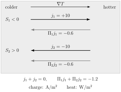
The equal-channel example in the exercises, with temperature increasing to the right. For $\partial_xT=1\,\mathrm{K/m}$, the electrical currents are $j_1=+10$ and $j_2=-10\,\mathrm{A/m^2}$. Since $\Pi_1=-0.060\,\mathrm V$ and $\Pi_2=+0.060\,\mathrm V$, both transported heat currents $\Pi_a j_a$ point left. They add $1.2\,\mathrm{W/m^2}$ of heat flow despite zero net charge current; the ordinary $\kappa_1+\kappa_2$ contribution is additional.

Nernst response and transverse heat transport

At nonzero field, use the full tensors and the actual thermal boundary condition. With $\mathbf B=B\hat{\mathbf z}$, in-plane isotropy, $\mathbf j=0$ and an imposed $\partial_yT=0$, write

$$\begin{aligned} \boldsymbol\sigma&= \begin{pmatrix}\sigma_{xx}&\sigma_{xy}\\-\sigma_{xy}&\sigma_{xx}\end{pmatrix},\\ \boldsymbol\alpha&= \begin{pmatrix}\alpha_{xx}&\alpha_{xy}\\-\alpha_{xy}&\alpha_{xx}\end{pmatrix}. \end{aligned}$$

Define the Nernst signal here as $N=\mathcal E_y/(-\partial_xT)=-S_{yx}$. Matrix inversion gives

$$N= \frac{\sigma_{xx}\alpha_{xy}-\sigma_{xy}\alpha_{xx}} {\sigma_{xx}^2+\sigma_{xy}^2}.$$

Some authors call $N/B$, usually in a weak-field limit, the Nernst coefficient; specify which quantity is reported. The measured signal contains both transverse thermoelectric response and Hall deflection of the compensating longitudinal field. If $\boldsymbol\alpha=c\boldsymbol\sigma$ for a scalar $c$, these cancel exactly. A nonzero Hall coefficient therefore need not imply a nonzero Nernst signal.

Thermally insulated sidewalls impose $j_{Q,y}=0$ rather than $\partial_yT=0$. A thermal Hall response then generates a transverse temperature gradient and changes the measured voltage. Eliminate the constrained components of the coupled equations for that geometry. Do not compare an adiabatic measurement directly with the isothermal-transverse formula without this step.

Berry curvature can contribute to transverse thermoelectricity, as developed by Xiao and collaborators (2006). In magnetic systems, microscopic equilibrium charge and energy circulations must be subtracted to obtain transport coefficients. Qin, Niu and Shi (2011) show the importance of energy-magnetization corrections for thermal Hall response. Applying a heat-current Kubo formula without the required corrections can violate reciprocity or generate an unphysical result. The microscopic current construction and geometric inputs are connected through Kubo Formula in Materials and Berry Curvature in Band Dynamics.

Power factor, figure of merit and measurement

For a homogeneous scalar material in the ordinary reciprocal, zero-field regime, define

$$\mathrm{PF}=S^2\sigma, \qquad ZT=\frac{S^2\sigma T}{\kappa_{\mathrm{tot}}}.$$

The denominator is the total open-circuit thermal conductivity in the same direction, at the same state and temperature. The power factor has units $\mathrm{W\,m^{-1}\,K^{-2}}$; $ZT$ is dimensionless. For $S=200\,\mu\mathrm{V/K}$, $\sigma=10^5\,\mathrm{S/m}$, $T=300\,\mathrm K$ and $\kappa_{\mathrm{tot}}=2\,\mathrm{W/(m\,K)}$, the power factor is $0.004\,\mathrm{W/(m\,K^2)}$ and $ZT=0.6$.

A high Seebeck coefficient with negligible conductivity need not provide useful power. Increasing carrier density, altering scattering or changing microstructure typically changes several coefficients at once; Snyder and Toberer (2008) discuss these competing material requirements. A scalar $ZT$ assembled from coefficients along different crystal axes has no standard device interpretation.

Nor is a peak material $ZT$ a device efficiency. Contacts, lead heat leaks, temperature-dependent coefficients, geometry, operating current and the finite temperature span must enter the device energy balance. Transverse devices, finite-field nonreciprocal configurations and strongly inhomogeneous samples require the appropriate tensor or terminal optimization, rather than automatic substitution into a scalar formula.

The relevant temperature difference is the one across the active sample. Lead thermopower, electrical loading and heat leaks can change the inferred coefficients; Transport Measurements explains how reversals and linearity tests help separate these effects. A small inferred electronic contribution is especially sensitive when obtained by subtracting two much larger heat flows.

Exercises

Distinguish zero field from zero current

At $T=300\,\mathrm K$, a reciprocal scalar electronic channel has $\sigma=10^5\,\mathrm{S/m}$, $\alpha=20\,\mathrm{A/(m\,K)}$ and $\bar\kappa_e=2\,\mathrm{W/(m\,K)}$. Find $S$, $\Pi$, $\kappa_e$ and the open-circuit field for $\partial_xT=10\,\mathrm{K/m}$. Does the coefficient set satisfy positivity?

Solution

The results are

$$\begin{aligned} S&=\alpha/\sigma=200\,\mu\mathrm{V/K},\\ \Pi&=TS=0.060\,\mathrm V,\\ \kappa_e&=2-300(20)^2/10^5\\ &=0.8\,\mathrm{W/(m\,K)},\\ \mathcal E_x&=S\partial_xT=0.002\,\mathrm{V/m}. \end{aligned}$$

At zero electrochemical field the heat current would be $-20\,\mathrm{W/m^2}$ and the charge current $-200\,\mathrm{A/m^2}$. At open circuit the compensating field contributes $+12\,\mathrm{W/m^2}$, leaving $-8\,\mathrm{W/m^2}$. Since $\kappa_e>0$ and $\sigma>0$, the scalar Onsager matrix is positive definite. “Zero field” in this comparison means zero electrochemical driving, not zero magnetic field.

Heat flow when thermopower cancels

At $300\,\mathrm K$, two independent channels have equal conductivities $5\times10^4\,\mathrm{S/m}$, thermopowers $S_1=-200\,\mu\mathrm{V/K}$ and $S_2=+200\,\mu\mathrm{V/K}$, and individual open-circuit thermal conductivities $\kappa_1=\kappa_2=0.6\,\mathrm{W/(m\,K)}$. Find the combined thermopower and electronic thermal conductivity under total $j=0$.

Solution

The conductivity-weighted thermopower is zero, but

$$\begin{aligned} \kappa_{\mathrm{bi}} &=300\,(2.5\times10^4)(4\times10^{-4})^2\\ &=1.2\,\mathrm{W/(m\,K)},\\ \kappa_e&=0.6+0.6+1.2 =2.4\,\mathrm{W/(m\,K)}. \end{aligned}$$

For a positive temperature gradient, $j_1=-\sigma_1S_1\nabla T$ and $j_2=-\sigma_2S_2\nabla T$ have equal and opposite signs. Their sum is zero without either channel being individually open-circuit. Imposing that stronger constraint would incorrectly discard the extra $1.2\,\mathrm{W/(m\,K)}$.

Mott thermopower with a declared energy scale

For electrons with $\Xi(\varepsilon)\propto(\varepsilon-E_c)^{3/2}$ near the chemical potential, take $\mu-E_c=0.20\,\mathrm{eV}$ and $T=20\,\mathrm K$. Estimate the diffusion thermopower and state the small parameter controlling the estimate.

Solution

The logarithmic derivative is $3/[2(\mu-E_c)]$. With $q=-e$,

$$S\simeq-\frac{\pi^2}{3}\frac{k_B}{e} \frac{k_BT}{\mu-E_c}\frac32 \simeq-3.66\,\mu\mathrm{V/K}.$$

Here $k_BT/(\mu-E_c)\simeq0.00862\ll1$. The result assumes smooth elastic transport on that energy scale and excludes drag. The exponent already includes the chosen state, velocity and lifetime weighting; it cannot be inferred from the density of states alone.

A Nernst signal requires the whole tensor

Let $\sigma=s_0\begin{pmatrix}2&1\\-1&2\end{pmatrix}$ and $\alpha=a_0\begin{pmatrix}3&4\\-4&3\end{pmatrix}$, with positive scale factors in their respective SI units. Find $\mathbf S$ and $N$ for $\partial_yT=0$. What would change if $\alpha=c\sigma$?

Solution

Direct multiplication gives

$$\begin{aligned} \mathbf S &=\frac{a_0}{5s_0} \begin{pmatrix}2&-1\\1&2\end{pmatrix} \begin{pmatrix}3&4\\-4&3\end{pmatrix}\\ &=\frac{a_0}{s_0} \begin{pmatrix}2&1\\-1&2\end{pmatrix}. \end{aligned}$$

Thus $N=-S_{yx}=a_0/s_0$. Using $\alpha_{xy}/\sigma_{xx}$ alone would instead give $2a_0/s_0$ and miss the compensating-field Hall term. If $\alpha=c\sigma$, then $\mathbf S=cI$ and $N=0$, even though $\sigma_{xy}$ can remain nonzero. A full thermodynamic model must also supply reciprocal cross-response and a thermal block satisfying positivity; this exercise only fixes the electrical open-circuit inversion.

References

• Herring, Conyers. “Theory of the Thermoelectric Power of Semiconductors.” Physical Review 96, 1163 (1954). doi:10.1103/PhysRev.96.1163. Nonequilibrium phonon drag and the reciprocal contribution to heat transport.
• Jonson, M., and G. D. Mahan. “Mott’s Formula for the Thermopower and the Wiedemann–Franz Law.” Physical Review B 21, 4223–4229 (1980). doi:10.1103/PhysRevB.21.4223. Microscopic consistency of electronic heat-current and thermoelectric formulas within specified scattering approximations.
• Qin, Tao, Qian Niu, and Junren Shi. “Energy Magnetization and the Thermal Hall Effect.” Physical Review Letters 107, 236601 (2011). doi:10.1103/PhysRevLett.107.236601. Magnetization corrections that distinguish transport heat current from equilibrium circulation.
• Snyder, G. Jeffrey, and Eric S. Toberer. “Complex Thermoelectric Materials.” Nature Materials 7, 105–114 (2008). doi:10.1038/nmat2090. Coupled material requirements for thermopower, conductivity and total thermal conductivity.
• Xiao, Di, Yugui Yao, Zhong Fang, and Qian Niu. “Berry-Phase Effect in Anomalous Thermoelectric Transport.” Physical Review Letters 97, 026603 (2006). doi:10.1103/PhysRevLett.97.026603. Orbital magnetization, anomalous thermoelectric response and reciprocal coefficients.