Current Noise and Fluctuations

Current noise measures correlations that the mean current leaves undetermined. Two conductors with the same conductance can have different transmission probabilities, transfer events or slow internal dynamics, and therefore different noise. The interpretation depends on which terminals, operator ordering, bandwidth and circuit the measurement resolves. The explicit partition formulas below concern stationary, elastic transport between normal reservoirs; interactions, superconducting conversion and time-dependent driving require their own transport models.

Required background. Noise Spectra supplies stationary correlations, Fourier measures and quantum ordering.

Helpful background. The Fluctuation–Dissipation Theorem supplies equilibrium response relations. Landauer–Büttiker Formalism fixes terminal signs and transmission channels, while Conductance Quantization explains their counting. Mesoscopic Transport treats charge-state kinetics and counting statistics; Transport Measurements establishes the experimental circuit and contact checks.

Current correlations and detector ordering

Let $I_\alpha$ be electric current directed out of reservoir $\alpha$ into the device, and subtract its stationary mean: $\delta I_\alpha=I_\alpha-\langle I_\alpha\rangle$. Use the two-sided ordered spectrum

$$S^>_{\alpha\beta}(\omega) =\int_{-\infty}^{\infty}dt\,e^{i\omega t} \langle\delta I_\alpha(t)\delta I_\beta(0)\rangle.$$

The half-anticommutator spectrum is

$$S^{\mathrm{sym}}_{\alpha\beta}(\omega) =\frac12\left[S^>_{\alpha\beta}(\omega) +S^>_{\beta\alpha}(-\omega)\right].$$

The swapped indices matter for distinct terminals. At each frequency these spectral matrices are Hermitian; cross entries may be complex. An autospectrum is real, and its symmetrized version is even in frequency. Do not impose those scalar properties on every cross entry.

An autocorrelation asks whether an unusually large current now tends to be followed by an unusually large current later. Its Fourier transform separates the time scales of those fluctuations. In quantum mechanics, interchanging the two current operators can change the answer: their order distinguishes energy available to a detector from energy the conductor can absorb.

For $\Omega>0$, $S^>_{\alpha\alpha}(+\Omega)$ describes the conductor’s ability to absorb energy $\hbar\Omega$; $S^>_{\alpha\alpha}(-\Omega)$ describes its ability to emit that energy. A weakly coupled detector initially in its ground state is excited by the latter. A symmetrized vacuum spectrum can be nonzero even when the conductor cannot excite that detector. The distinction follows from the ordering of the detector transition probability [Clerk et al., 2010]; a specific detector need not return the symmetrized spectrum [Lesovik and Loosen, 1997].

The units are current squared times time. A finite classical measurement has a transfer function $H(\omega)$ and, for one channel without additional detector noise,

$$\operatorname{Var}I_{\mathrm{filtered}} =\int_{-\infty}^{\infty}\frac{d\omega}{2\pi} |H(\omega)|^2S^{\mathrm{sym}}(\omega).$$

Here the use of the symmetrized spectrum presumes the corresponding classical-record calibration. A white spectrum over an ideal infinite bandwidth does not define a finite instantaneous variance.

The factor of two is a convention

Define a separate symbol $\mathcal S(\omega)=2S^{\mathrm{sym}}(\omega)$ for the frequently used transport normalization [Blanter and Büttiker, 2000, footnote 4]. For a scalar conductance $G$, the low-frequency limits are:

Quantity	Two-sided $S^{\mathrm{sym}}(0)$	Doubled $\mathcal S(0)$
Equilibrium, classical limit	$2k_BT G$	$4k_BT G$
Zero-temperature partition noise	$\lvert qI\rvert F$	$2\lvert qI\rvert F$

This translates the shot-noise formulas in the conductance and sequential-transport prerequisites. It is unrelated to spin degeneracy. Each resolved spin channel will be counted explicitly below.

For a classical autospectrum reported per hertz, a one-sided density is $P_1(f)=2S^{\mathrm{sym}}(2\pi f)$ for $f>0$, with variance $\int_0^\infty df\,|H(2\pi f)|^2P_1(f)$. The change of measure $d\omega/(2\pi)=df$ explains why no additional numerical $2\pi$ multiplies this density. Folding a classical spectrum is not a rule for replacing an ordered quantum emission spectrum.

Equilibrium noise and terminal dissipation

For the terminal admittance $I_\alpha(\omega)=\sum_\beta Y_{\alpha\beta}(\omega)V_\beta(\omega)$, use the electrochemical voltage convention of the Landauer page. The equilibrium matrix relation is

$$\begin{aligned} S^{\mathrm{sym}}(\omega) &=\hbar\omega\coth\!\left(\frac{\hbar\omega}{2k_BT}\right)Y_H(\omega),\\ Y_H&=\frac{Y+Y^\dagger}{2}. \end{aligned}$$

The response and noise must refer to the same complete terminal problem, including displacement currents where needed. $Y_H$ is the dissipative Hermitian part that enters the time-averaged electrical power. In the classical dc limit, with real conductance matrix $G$,

$$S^{\mathrm{sym}}(0)=k_BT(G+G^{\mathsf T}).$$

For a nonreciprocal conductor this is not the componentwise formula $2k_BT G_{\alpha\beta}$. The latter would generally fail even the symmetry required of a zero-frequency covariance. Exercise 2 makes the distinction explicit.

In thermal equilibrium the ordered spectra also satisfy

$$S^>_{\beta\alpha}(-\omega) =e^{-\hbar\omega/(k_BT)}S^>_{\alpha\beta}(\omega).$$

Fluctuation–dissipation relations derive this thermal identity. A dc-biased stationary conductor need not obey it, even when its average current is independent of time.

Partition noise from occupied incoming channels

Consider a coherent two-terminal normal conductor with independent Fermi reservoirs. Let $q=-e$, $e>0$, and let $\tau_n(E)$ be its resolved transmission eigenvalues. The one-particle description must be valid over the transport window; it is not a general formula for an interacting conductor. The scattering approach separates fluctuations of incident occupation from partition at the device [Büttiker, 1992].

For a single channel and energy cell, let $X$ count net transferred particles from left to right in one available incident state. The left-only occupation has probability $f_L(1-f_R)$ and permits $X=+1$ with probability $\tau$; the right-only occupation similarly permits $X=-1$. With both incident states filled, Pauli exclusion leaves zero net transfer. Therefore

$$\begin{aligned} \langle X\rangle&=\tau(f_L-f_R),\\ \langle X^2\rangle&=\tau[f_L(1-f_R)+f_R(1-f_L)]. \end{aligned}$$

Subtracting the square of the mean gives

$$\operatorname{Var}X ={}\tau[f_L(1-f_L)+f_R(1-f_R)] +\tau(1-\tau)(f_L-f_R)^2.$$

Over a long counting time $t$, an energy interval $dE$ supplies $t\,dE/h$ attempts per resolved channel. The variance of transferred charge grows as $tS^{\mathrm{sym}}(0)$ in our normalization. This yields

$$S^{\mathrm{sym}}(0) =\frac{q^2}{h}\int dE\sum_n\operatorname{Var}X_n(E),$$

where each variance is the expression just derived, with $\tau=\tau_n(E)$. Its first term survives at equilibrium. The second is partition noise and vanishes for each closed or perfectly open channel. Thus a noiseless zero-temperature open channel can carry nonzero current. The absence of its partition noise does not remove finite-temperature occupation fluctuations.

At zero temperature, let $\mathcal W$ be the interval between the two chemical potentials. Comparing with the mean current gives

$$\begin{gathered} F_{\mathcal W} =\frac{\int_{\mathcal W}dE\sum_n\tau_n(E)[1-\tau_n(E)]} {\int_{\mathcal W}dE\sum_n\tau_n(E)},\\ S^{\mathrm{sym}}(0)=|qI|F_{\mathcal W}. \end{gathered}$$

The ratio is defined only for nonzero transmitted current. In infinitesimal bias, or when the eigenvalues are effectively constant throughout $\mathcal W$,

$$F=\frac{\sum_n\tau_n(1-\tau_n)}{\sum_n\tau_n}.$$

Then $0\leq F\leq1$, with the Poisson value approached for weak transmissions. Conductance fixes $\sum_n\tau_n$, whereas noise additionally constrains $\sum_n\tau_n^2$. Neither generally identifies the complete transmission distribution.

The thermal-to-shot-noise crossover

Assume equal reservoir temperature and transmissions constant over both the thermal and bias windows. Define $D=|\mu_L-\mu_R|=|q\Delta V|$, $g=q^2/h$ and $G=g\sum_n\tau_n$. The Fermi integrals obey

$$\begin{gathered} \int dE\,f(1-f)=k_BT, \\ \int dE\,(f_L-f_R)^2 =D\coth\!\left(\frac{D}{2k_BT}\right)-2k_BT. \end{gathered}$$

Inserting them into the occupation result and using $GF=g\sum_n\tau_n(1-\tau_n)$ gives the crossover in the stated normalization, for $G>0$:

$$S^{\mathrm{sym}}(0)=2k_BT G {}+GF \left[D\coth\!\left(\frac{D}{2k_BT}\right)-2k_BT\right].$$

If all channels are closed, the noise is zero directly from the occupation formula. At small $D$, the bracket is $D^2/(6k_BT)+O(D^4/(k_BT)^3)$, so equilibrium noise is recovered smoothly. At zero temperature with nonzero bias it tends to $D$, recovering partition shot noise. A full Poisson term added to full Johnson noise does not describe the intermediate region. This result is the constant-transmission specialization of the scattering expression [Blanter and Büttiker, 2000].

An excess spectrum subtracts a declared reference, for example $S(V,T)-S(0,T)$. It is different from the absolute spectrum; a difference of spectra need not itself be a positive spectral matrix. Electron heating or a bias-dependent transmission also changes the reference comparison, so a fitted excess slope cannot automatically be read as a transfer charge.

Terminal cross correlations and the circuit

In a closed two-terminal dc measurement with no accumulating device charge, $\delta I_1=-\delta I_2$ at zero frequency. Hence

$$S^{\mathrm{sym}}(0) =S_{11}^{\mathrm{sym}}(0) \begin{pmatrix}1&-1\\-1&1\end{pmatrix}.$$

Changing the sign assigned to one current changes the sign of its cross spectrum. State both lead directions before interpreting a measured anticorrelation.

For elastic normal fermion scattering with independent equilibrium reservoirs, the low-frequency correlations between distinct lead currents are nonpositive in this common-direction convention [Büttiker, 1992]. This conclusion has hypotheses: fluctuating voltage probes, interactions, superconducting conversion and external feedback change the transport problem. Positive measured correlations alone do not establish pairs, entanglement or a particle’s exchange statistics.

At finite frequency, particle currents can charge the device. Their sum need not vanish instantaneously; the complete measured terminal currents involve the electric field, gates and displacement current. A dc conductance matrix with a frequency label attached is not a complete finite-frequency circuit model. This is also why a zero-average-current probe does not have identically zero current fluctuations.

Finite-frequency emission is detector dependent

An instructive limit is a normal tunnel conductor at zero temperature, with constant conductance $G$ and energy bias $D$. To leading order in its small transmissions, the ordered spectrum at frequencies below internal and circuit dynamical scales is

$$S^>(\omega) =G\left[(\hbar\omega+D)_+ +(\hbar\omega-D)_+\right],$$

where $(x)_+=\max(x,0)$. The two terms count available occupied-to-empty energy intervals for opposite transfer directions. For a detector frequency $\Omega>0$,

$$S_{\mathrm{em}}(\Omega) \equiv S^>(-\Omega) =G(D-\hbar\Omega)_+.$$

Emission stops when one transfer cannot supply the detector quantum. Absorption and symmetrized noise need not stop there. At equilibrium and zero temperature, $S^>(+\Omega)=2G\hbar\Omega$, $S^>(-\Omega)=0$, and $S^{\mathrm{sym}}(\Omega)=G\hbar\Omega$.

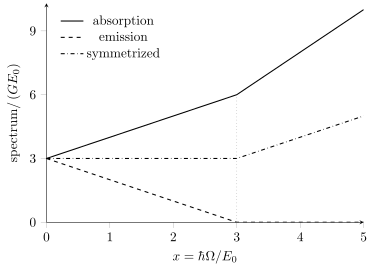
Zero-temperature tunnel benchmark with $D=3E_0$. The spectrum is expressed in units $GE_0$, and $x=\hbar\Omega/E_0>0$. Above $x=3$, a ground-state detector cannot extract a quantum from a single transfer, although the symmetrized spectrum continues to grow. The three curves correspond to different operator orderings, not three independent noise sources to add together.

The detector coupling, its initial population and its own response determine which combination is registered [Lesovik and Loosen, 1997; Clerk et al., 2010]. The cutoff above belongs to this tunnel model. Heating, an external drive, correlated transfers or a different electromagnetic environment can supply additional energy; the expression is not a universal bound on every biased device.

Charge inference and slow noise

For independent rare events carrying signed charges $q_j$ at rates $\Gamma_j$,

$$\begin{aligned} I&=\sum_jq_j\Gamma_j,\\ S^{\mathrm{sym}}(0)&=\sum_jq_j^2\Gamma_j. \end{aligned}$$

Consequently the fitted ratio $\mathcal S/(2|I|)$ need not equal any one event charge. Correlated waiting times and charge-state constraints change these Poisson cumulants; Mesoscopic Transport derives the corresponding counting statistics.

Noise can constrain quasiparticle charge once a transport model, regime and competing mechanisms are controlled. The relevant platform derivations are Fractional Quantum Hall Effect for fractional edge transport and Proximity and Andreev Physics for electron–hole conversion. Replacing $e$ by a proposed charge in a normal-conductor formula is not sufficient. Charge, transfer multiplicity and exchange statistics are distinct inferences.

Slow switching also produces noise without changing the microscopic carrier charge. A stationary Markov switch between currents $I_a,I_b$, with occupation probabilities $p_a,p_b$ and relaxation rate $\Gamma=\Gamma_{a\to b}+\Gamma_{b\to a}$, gives

$$S^{\mathrm{sym}}(\omega) =\frac{2p_ap_b(I_a-I_b)^2\Gamma}{\Gamma^2+\omega^2}.$$

It is a Lorentzian from an exponential correlation, not a white partition spectrum. An ensemble of relaxation rates can produce an approximate $1/f$ range; physical cutoffs and stationarity still matter. See 1/f Noise for that mechanism and its limits.

Cross-correlation techniques reject independent amplifier noise, but retain shared pickup and physical backaction. Even background subtraction requires the amplifier–sample correlations to be negligible or separately determined. Transport Measurements explains the circuit, and Noise Spectra explains detector filtering.

Exercises

1. A finite-temperature partition measurement

Two resolved channels have $\tau_1=0.2$, $\tau_2=0.7$, and $D=6k_BT$. Find $G$, the zero-temperature Fano factor, the equilibrium contribution, excess noise and full noise. Express spectra in units $gk_BT$, and translate the full result to the doubled convention.

Solution

Here $G=0.9g$ and $\sum_n\tau_n(1-\tau_n)=0.16+0.21=0.37$, so $F=37/90$. The equilibrium contribution is $1.8gk_BT$. The excess is $0.37[6\coth(3)-2]gk_BT$, or $1.491033\,gk_BT$. Thus

$$\begin{aligned} S^{\mathrm{sym}}(0)&=3.291033\,gk_BT,\\ \mathcal S(0)&=6.582066\,gk_BT. \end{aligned}$$

The finite-temperature excess is not $|qI|F$: the latter would give $2.22gk_BT$. The subtraction of $2k_BT$ inside the crossover bracket is consequential.

2. Equilibrium noise in a directed network

Use the four-terminal network $1\to2\to3\to4\to1$ from the Landauer article, with one channel per link and common temperature. Its dc currents obey $I_\alpha=g(V_\alpha-V_{\alpha-1})$, with cyclic indices. Find the equilibrium noise matrix and its eigenvalues. Explain why $2k_BT G$ is incorrect.

Solution

Adding $G$ and its transpose gives

$$\frac{S^{\mathrm{sym}}(0)}{k_BTg} =\begin{pmatrix} 2&-1&0&-1\\ -1&2&-1&0\\ 0&-1&2&-1\\ -1&0&-1&2 \end{pmatrix}.$$

Its eigenvalues are $0,2,2,4$. The uniform zero mode expresses current conservation; every other eigenvalue is nonnegative. The matrix $2G/g$ is not symmetric and so cannot be this dc covariance. Noise constrains the dissipative part of a nonreciprocal response, not its full directional information.

3. A detector above the emission cutoff

For the zero-temperature tunnel benchmark take $D=3E_0$. Evaluate absorption, emission and symmetrized spectra at $\hbar\Omega=2E_0$ and $4E_0$, in units $GE_0$. Also compute the symmetrized excess relative to zero-bias equilibrium.

Solution

At $2E_0$, the absorption and emission values are $5$ and $1$, so their half-sum is $3$. At $4E_0$, they are $8$ and $0$, giving half-sum $4$. The corresponding equilibrium symmetrized values are $2$ and $4$; the excess values are therefore $1$ and $0$.

A ground-state detector can be excited in the first case, but not the second within this model. The nonzero second symmetrized value represents absorption/vacuum fluctuations, not available emitted power.

4. An inferred charge that no event carries

Independent transfers in the same current direction carry charge magnitudes $e$ at rate $3\gamma$ and $2e$ at rate $\gamma$. What charge would a fit to $\mathcal S=2q_{\mathrm{fit}}|I|$ report? Does it establish a fractional elementary transfer?

Solution

The current magnitude is $5e\gamma$, whereas $S^{\mathrm{sym}}(0)=7e^2\gamma$ and $\mathcal S(0)=14e^2\gamma$. Hence $q_{\mathrm{fit}}=7e/5$, although the only events carry $e$ and $2e$. The second cumulant weights charges quadratically and the mean weights them linearly. A single fitted ratio therefore cannot identify an event distribution, still less an exchange statistic.

References

• Blanter, Ya. M., and Büttiker, M., “Shot noise in mesoscopic conductors,” Physics Reports 336, 1–166 (2000), doi:10.1016/S0370-1573(99)00123-4, author preprint — transport normalization, partition noise and thermal crossover.
• Büttiker, M., “Scattering theory of current and intensity noise correlations in conductors and wave guides,” Physical Review B 46, 12485–12507 (1992), doi:10.1103/PhysRevB.46.12485 — reservoir occupation, scattering and terminal correlations.
• Clerk, A. A., Devoret, M. H., Girvin, S. M., Marquardt, F., and Schoelkopf, R. J., “Introduction to quantum noise, measurement, and amplification,” Reviews of Modern Physics 82, 1155–1208 (2010), doi:10.1103/RevModPhys.82.1155, author preprint — ordered spectra, detector transitions and quantum measurement.
• Lesovik, G. B., and Loosen, R., “On the detection of finite-frequency current fluctuations,” JETP Letters 65, 295–299 (1997), doi:10.1134/1.567363, author preprint — ordering selected by a finite-frequency detector; the linked preprint was uploaded in 2008.