Magnetoresistance

Magnetoresistance is a change in longitudinal electrical resistance when a magnetic field changes the carrier trajectories, scattering, quantum coherence or material state. Its sign and shape do not identify a unique mechanism. Even the starting classical model has a useful surprise: a homogeneous, isotropic one-carrier Drude conductor has zero intrinsic dc magnetoresistance despite a field-dependent longitudinal conductivity. The Hall field restores the cancellation when the conductivity tensor is inverted under the correct boundary condition.

The cancellation and a two-carrier example below separate changes of conductivity from changes of the measured resistivity. Boltzmann transport develops the kinetic theory, weak localization explains interference corrections, and spintronics treats spin-dependent devices. Transport measurements explains contacts and conversion of terminal voltages.

Required background. Hall Effect supplies the tensor convention and the distinction between an applied field and an open transverse circuit.

Helpful background. Boltzmann Transport supplies orbit and scattering dependence; Transport Measurements supplies terminal and geometry checks; Weak Localization supplies coherence scales; Spintronics supplies magnetic mechanisms; Weyl and Dirac Semimetals supplies anomaly conditions; Data Interpretation Pitfalls supplies inference tests.

Longitudinal resistance and the comparison state

For a material resistivity component along the imposed current, define

$$\begin{aligned} \mathrm{MR}(B)&=\frac{\rho_{xx}(B)-\rho_0}{\rho_0},\\ \rho_0&=\rho_{xx}(0)>0. \end{aligned}$$

The percentage is $100\,\mathrm{MR}$. Temperature, gate voltage, current direction, sample geometry and preparation protocol must be specified. Field-induced changes in magnetic order, carrier density or phase are part of the measured response, but a comparison that permits them is different from a calculation that holds those quantities fixed. In a hysteretic system, label the sweep branch and the zero-field reference state. If the reference is superconducting with $\rho_0=0$, this ratio is undefined; report the resistance itself or a declared finite normal-state reference.

“Longitudinal” can describe the voltage component along the current or the alignment of the field. Here $\rho_{xx}$ is always the former. Transverse magnetoresistance uses $\mathbf B\perp\mathbf j$; longitudinal magnetoresistance uses $\mathbf B\parallel\mathbf j$. A transverse-field experiment still measures a longitudinal resistivity change, not the Hall voltage.

For a homogeneous bar with uniform current, $R_{xx}=\rho_{xx}L/A$ and a field-independent geometric factor cancels in the ratio. When current paths or conducting dimensions change with field, the measured ratio $[R(B)-R(0)]/R(0)$ need not equal the intrinsic material ratio. State whether the reported object is a bulk resistivity, sheet resistance or specified terminal resistance.

In equilibrium linear response, Onsager–Casimir reciprocity gives

$$\rho_{ij}(\mathbf B,\mathbf M) =\rho_{ji}(-\mathbf B,-\mathbf M),$$

where $\mathbf M$ represents time-reversal-odd order; any other such parameters must also reverse. Thus a nonmagnetic homogeneous diagonal resistivity is even in $B$. Reversing only the applied field on a hysteresis branch need not reach the time-reversed state. Nor does this diagonal tensor relation make every four-terminal resistance even without exchanging current and voltage terminals appropriately.

Tensor inversion and the zero Drude benchmark

Take $\mathbf B=B\hat{\mathbf z}$ and a uniform isotropic in-plane medium. Use $j_i=\sigma_{ij}E_j$ and $E_i=\rho_{ij}j_j$. In the absence of a symmetric off-diagonal contribution,

$$\begin{aligned} \boldsymbol\sigma&= \begin{pmatrix}\sigma_{xx}&\sigma_{xy}\\-\sigma_{xy}&\sigma_{xx}\end{pmatrix},\\ \rho_{xx}&=\frac{\sigma_{xx}}{\sigma_{xx}^2+\sigma_{xy}^2}. \end{aligned}$$

This is the open-transverse-circuit result $j_y=0$. It is generally different from $1/\sigma_{xx}$, which would describe the ratio $E_x/j_x$ with $E_y=0$ and transverse current allowed. For anisotropic media, invert the actual full tensor rather than substituting into this isotropic formula.

The one-carrier Drude result, with signed charge $q$, constant density $n$, mass $m^*$ and relaxation time $\tau$, is

$$\begin{aligned} \sigma_0&=\frac{nq^2\tau}{m^*}, &\beta&=\frac{qB\tau}{m^*},\\ \sigma_{xx}&=\frac{\sigma_0}{1+\beta^2}, &\sigma_{xy}&=\frac{\sigma_0\beta}{1+\beta^2}. \end{aligned}$$

Consequently,

$$\rho_{xx}(B)=\frac1{\sigma_0}, \qquad \rho_{yx}(B)=\frac{B}{nq}.$$

The Lorentz force bends motion but does no work. In this model the transverse Hall field exactly compensates its deflection in the steady drift, leaving the required longitudinal field unchanged. Treating the decrease of $\sigma_{xx}$ as increased measured resistivity would predict a spurious $\mathrm{MR}=\beta^2$.

The cancellation assumes a homogeneous dc response, open transverse circuit, one isotropic parabolic carrier population and field-independent parameters. It does not forbid magnetoresistance in a material or in a finite device. Changes in those assumptions must be identified explicitly rather than hidden in a fitted field-dependent mobility.

Two-carrier compensation and the saturation scale

An instructive departure retains classical isotropic bands but includes electrons of density $n$ and holes of density $p$. Their positive mobilities are $\mu_e$ and $\mu_h$, in $\mathrm{m^2\,V^{-1}\,s^{-1}}$, so $\mu B$ is dimensionless in SI. Assume independent carrier channels, fixed densities and mobilities, and a nonquantizing transverse field.

Conductivities add before inversion. The two-carrier Hall construction gives the longitudinal result

$$\begin{aligned} S&=n\mu_e+p\mu_h,\\ \mathcal D(B)&=S^2+(p-n)^2\mu_e^2\mu_h^2B^2,\\ \rho_{xx}(B)&= \frac{S+(n\mu_h+p\mu_e)\mu_e\mu_hB^2} {e\mathcal D(B)}. \end{aligned}$$

Here $e>0$ and $\rho_0=1/(eS)$. Subtracting this zero-field value yields

$$\mathrm{MR}(B)= \frac{np\mu_e\mu_h(\mu_e+\mu_h)^2B^2} {\mathcal D(B)}.$$

Every factor in the numerator is nonnegative. The result vanishes if either carrier population is absent and becomes especially simple at exact compensation:

$$n=p:\qquad \mathrm{MR}(B)=\mu_e\mu_h B^2.$$

Compensation therefore permits a large nonsaturating classical magnetoresistance without a change in density or scattering. For example, $\mu_e=2\,\mathrm{m^2/(V\,s)}$, $\mu_h=0.5\,\mathrm{m^2/(V\,s)}$ and $B=5\,\mathrm T$ give $\mathrm{MR}=25$, or $2500\%$. Large percentage values alone are not evidence for a quantum mechanism.

The two species share one transverse electric field, but their charges and longitudinal drift velocities have opposite signs. The field that cancels the Lorentz deflection of one species cannot cancel that of the other. Only their total transverse charge current must vanish; each population can retain transverse motion. Solving the two force-balance equations together changes the longitudinal field required to carry a fixed total current.

For $p\ne n$, the denominator changes behavior at

$$B_c=\frac{n\mu_e+p\mu_h}{|p-n|\mu_e\mu_h}.$$

The model saturates only when $|B|\gg B_c$, within its range of validity. Near compensation this can be much larger than both inverse mobilities. Failure to observe saturation in a finite field window therefore does not establish exact compensation. Conversely, a high-field saturation formula is unreliable if Landau quantization, magnetic breakdown, a field-induced transition or changing carrier parameters intervenes first.

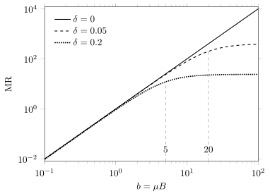
Equal mobilities give $\mathrm{MR}=(1-\delta^2)b^2/(1+\delta^2b^2)$, where $b=\mu B$ and $\delta=(p-n)/(p+n)$. All three curves are nearly quadratic at small $b$. The imbalanced curves bend toward saturation near $b=1/|\delta|$, which moves to arbitrarily large field as compensation improves. These are exact curves of the classical model; continuation to large $b$ assumes that quantization and changing material parameters remain negligible.

Fit the longitudinal and Hall components together, with consistent tensor inversion. The Hall curve supplies different density/mobility combinations, but even a simultaneous fit may have strongly correlated parameters over a restricted field range. Independent density and Fermi-surface information remains valuable.

Fermi-surface orbits and field alignment

In a general crystal, the field samples velocity correlations along Fermi-surface orbits. The velocity-history formulation is derived in Boltzmann Transport. Closed and open orbits, scattering anisotropy and multiple pockets can produce different angular dependences and high-field limits. The one-band cancellation is therefore a benchmark to test, not a general prediction from the word “metal.”

Even $\mathbf B\parallel\mathbf j$ does not universally eliminate orbital magnetoresistance: a crystal velocity need not be parallel to crystal momentum, and different components of the distribution remain coupled. Pal and Maslov (2010) give the conditions for this effect within a scalar relaxation-time treatment. Anisotropy alone is insufficient; a simple ellipsoidal parabolic band with a constant relaxation time still has field-independent intrinsic diagonal resistivity. More general orbit dependence or scattering is needed.

Keep the classical bending scale and the quantization scale separate. For a parabolic pocket, $\omega_c\tau_{\mathrm{tr}}\sim1$ means substantial bending during a transport lifetime. Resolved Landau levels instead depend on $\hbar\omega_c$ relative to temperature and spectral broadening, while the quantum limit requires occupation of only the lowest relevant levels. The transport and quantum lifetimes can differ greatly. Fermi Surface and Landau Levels supply the orbit and spectrum tests.

Kohler scaling and its assumptions

Suppose the Fermi surface, carrier densities and normalized collision operator remain fixed as temperature varies, while all relevant relaxation rates share one scale $1/\tau(T)$. The semiclassical conductivity then has the schematic structure

$$\boldsymbol\sigma(B,T)=\tau(T)\, \mathcal S\big(B\tau(T)\big).$$

Material constants supply the units of the argument. Inverting the tensor gives $\rho_0(T)\propto1/\tau(T)$ and hence the conventional Kohler form

$$\frac{\Delta\rho(B,T)}{\rho_0(T)} =F\!\left(\frac{B}{\rho_0(T)}\right).$$

The horizontal axis has units; the function incorporates the fixed conversion factors. Use consistent field and resistivity units across temperatures. A collapse is evidence for compatible single-scale transport, and can occur in a multiband system when mobility ratios and carrier populations stay fixed. It does not prove that only one band conducts or that one microscopic scattering process exists.

A failure to collapse says that at least one scaling assumption fails. Possible causes include changing carrier density, changing ratios of scattering rates, Fermi-surface reconstruction, anisotropic scattering changes, quantum corrections and inhomogeneity. Xu and collaborators (2021) demonstrate the role of temperature-dependent carrier density in a generalized scaling analysis. Kohler violation by itself is insufficient evidence for non-Fermi-liquid behavior. Normalizing every curve by an unconstrained adjustable scale can also hide the physics that the test was meant to examine.

Magnetic orientation, interference and other candidates

In a uniaxial magnetic conductor, a useful lowest-order symmetric anisotropic-resistivity model is

$$\begin{aligned} \rho_{ij}^{\mathrm{sym}} &=\rho_\perp\delta_{ij}+\Delta\rho\,m_i m_j,\\ \Delta\rho&=\rho_\parallel-\rho_\perp, \end{aligned}$$

where $\mathbf m$ is the unit magnetization direction. For in-plane $\mathbf m=(\cos\theta,\sin\theta)$ and $j_y=0$,

$$\begin{aligned} \rho_{xx}&=\rho_\perp+\Delta\rho\cos^2\theta,\\ \rho_{yx}^{\mathrm{sym}}&=\Delta\rho\sin\theta\cos\theta. \end{aligned}$$

The second expression is the planar Hall signal of this model. It is symmetric in the tensor indices and unchanged by $\mathbf m\mapsto-\mathbf m$; it is distinct from an antisymmetric Hall response. The angle is the magnetization angle, which need not follow the applied field in the presence of anisotropy or domains. Crystalline corrections can add harmonics. Spintronics distinguishes this anisotropic magnetoresistance from metallic spin valves, tunnel-junction magnetoresistance and interfacial spin Hall magnetoresistance.

Different mechanisms can produce similar curve shapes. Their characteristic scales and independent observables distinguish them:

Candidate	Evidence to seek	A competing explanation to test
Orbital or multiband response	Joint Hall and longitudinal fits, mobility scales, orbit-angle dependence	Field-dependent populations or nonuniform current
Weak localization or antilocalization	Diffusive/coherent window, temperature dependence and appropriate spin-channel field scales	Classical background or interaction corrections
Magnetic scattering or spin-dependent devices	Magnetic state, relative layer angles, switching and history	Contact effects, heating or orbital response
Quantum-limit transport	Independently constrained filling and resolved level scales	Classical compensation or mobility inhomogeneity
Anomaly-related longitudinal response	Appropriate Weyl pockets and relaxation regime, angular and sample-geometry controls	Current jetting or other negative magnetoresistance mechanisms

The usual weak-localization correction reduces zero-field conductivity; suppressing it with an orbital field can give negative magnetoresistance. Spin–orbit coupling can reverse the interference correction. Fit the appropriate conductivity correction after tensor conversion, as explained by Weak Localization. A low-field cusp alone does not determine the number or topology of conducting channels.

Likewise, an approximately linear nonsaturating response is not unique to the quantum limit. Parish and Littlewood (2003) construct a classical inhomogeneous-conductor mechanism in which spatial variations and local Hall response reshape current paths. Its existence is a counterexample to uniqueness, not an assignment of that mechanism to every linear trace.

Current distribution and the limit of subtraction

Current jetting is particularly consequential in high-mobility samples with strong field-induced conductivity anisotropy. Current injected through finite contacts can concentrate into narrow paths. A voltage pair away from those paths may register a decreasing voltage even when the intrinsic resistivity along the field does not decrease. Dos Reis and collaborators (2016) demonstrate the resulting dependence on current injection and voltage-contact placement.

The local diffusive forward problem is

$$\boldsymbol\nabla\cdot \left[\boldsymbol\sigma(\mathbf r,B) \boldsymbol\nabla V(\mathbf r)\right]=0,$$

with imposed current-contact flux and insulating boundary conditions elsewhere. The measured voltage samples the resulting potential at the probe contacts. For uniform current this reduces to the familiar geometric conversion; an anisotropic or inhomogeneous sample can require solving the boundary problem. Transport Measurements explains the geometry and contact conditions.

Field symmetrization removes an odd Hall admixture only when the intended longitudinal part is even and the paired states are appropriate. It does not remove an even current-redistribution artifact. Useful checks include multiple voltage pairs, altered current-contact geometry, aspect-ratio dependence, both field directions and sweep branches, small-angle rotation, and current-amplitude dependence. These controls test different failure modes; no single one establishes an intrinsic response.

Finally, subtracting a fitted “ordinary background” does not isolate a unique new mechanism. Independent parallel channels add in conductivity, while collision mechanisms enter the kinetic operator; their effects need not add as scalar resistivities. Specify which object is being modeled and why the components can be combined in that way. A negative residual after an arbitrary positive background subtraction has no standalone microscopic meaning. Weyl and Dirac Semimetals develops the additional requirements for an anomaly interpretation.

Exercises

A conductivity change without magnetoresistance

For a one-carrier Drude system with $|\beta|=3$, find $\sigma_{xx}/\sigma_0$, $|\sigma_{xy}|/\sigma_0$, and the true $\rho_{xx}/\rho_0$. What false magnetoresistance follows from using $1/\sigma_{xx}$?

Solution

The conductivities are $\sigma_{xx}=\sigma_0/10$ and $|\sigma_{xy}|=3\sigma_0/10$. The denominator of the inverse tensor is $\sigma_0^2/10$, so $\rho_{xx}=1/\sigma_0=\rho_0$. The true magnetoresistance is zero. The incorrect reciprocal gives $10\rho_0$, hence a false $\mathrm{MR}=9$ or $900\%$. The difference comes from imposing different transverse boundary conditions.

Near compensation is not exact compensation

Take equal mobilities $\mu_e=\mu_h=\mu$ and define $\delta=(p-n)/(p+n)$. Derive the magnetoresistance as a function of $b=\mu B$. Evaluate it for $\delta=0.05$, $\mu=1\,\mathrm{m^2/(V\,s)}$ and $B=5\,\mathrm T$, and find the crossover and saturation values.

Solution

Since $4np=(p+n)^2(1-\delta^2)$, the two-carrier formula becomes

$$\mathrm{MR}=\frac{(1-\delta^2)b^2}{1+\delta^2b^2}.$$

At the specified field, $b=5$ and $\mathrm{MR}=24.9375/1.0625\simeq23.4706$, or about $2347\%$. The denominator crosses over at $|b|=1/|\delta|=20$, hence $B_c=20\,\mathrm T$. The limiting ratio is $(1-\delta^2)/\delta^2=399$. A nonsaturating-looking trace below $5\,\mathrm T$ is therefore compatible with a nonzero imbalance. The asymptotic prediction is conditional on the model remaining valid at much higher fields.

A conventional failure of Kohler collapse

At every temperature let a classical two-carrier system be compensated, with $n=p=N(T)$ and equal mobilities $\mu(T)$. Show that at a fixed plotted value $X=B/\rho_0(T)$ the magnetoresistance depends on $N(T)$, even though no exotic scattering is present.

Solution

Here $\rho_0=1/[2eN(T)\mu(T)]$ and $\mathrm{MR}=\mu(T)^2B^2$. Therefore

$$X=2eN\mu B, \qquad \mathrm{MR}=\frac{X^2}{4e^2N(T)^2}.$$

Doubling $N$ reduces the magnetoresistance at fixed $X$ by four. The mobility scale has canceled, but the changing population has not. The example violates the fixed-density assumption of conventional Kohler scaling and requires no change in the character of the quasiparticles.

A planar transverse signal without antisymmetric Hall response

Let $\rho_\perp=100$ and $\rho_\parallel=110$ in the same resistivity units. Compute the in-plane resistivity tensor at $\theta=45^\circ$, its eigenvalues, and its value under magnetization reversal. Explain why this transverse voltage alone does not establish an ordinary or anomalous Hall effect.

Solution

With $\Delta\rho=10$,

$$\boldsymbol\rho^{\mathrm{sym}} =\begin{pmatrix}105&5\\5&105\end{pmatrix}.$$

The eigenvalues are $110$ along $\mathbf m$ and $100$ perpendicular to it; dissipation is positive. The off-diagonal entries are equal. Magnetization reversal sends $\theta\mapsto\theta+\pi$ and leaves every entry unchanged. Thus $E_y=5j_x$ for an open transverse circuit is fully explained by a symmetric anisotropic tensor. An antisymmetric Hall component requires its own tensor/parity analysis; a transverse voltage by itself does not supply one.

References

• Dos Reis, R. D., M. O. Ajeesh, N. Kumar, F. Arnold, C. Shekhar, M. Naumann, M. Schmidt, M. Nicklas, and E. Hassinger. “On the Search for the Chiral Anomaly in Weyl Semimetals: The Negative Longitudinal Magnetoresistance.” New Journal of Physics 18, 085006 (2016). doi:10.1088/1367-2630/18/8/085006; arXiv:1606.03389. Current jetting, contact dependence and the distinction between terminal voltage and intrinsic longitudinal resistivity.
• Pal, H. K., and D. L. Maslov. “Necessary and Sufficient Condition for Longitudinal Magnetoresistance.” Physical Review B 81, 214438 (2010). doi:10.1103/PhysRevB.81.214438; arXiv:1003.2997. Fermi-surface conditions for orbital longitudinal magnetoresistance within the stated relaxation-time approximation.
• Parish, M. M., and P. B. Littlewood. “Non-saturating Magnetoresistance in Heavily Disordered Semiconductors.” Nature 426, 162–165 (2003). doi:10.1038/nature02073; arXiv:cond-mat/0312020. A classical inhomogeneity mechanism for approximately linear nonsaturating magnetoresistance.
• Xu, Jing, Fei Han, Ting-Ting Wang, Laxman R. Thoutam, Samuel E. Pate, Mingda Li, Xufeng Zhang, Yong-Lei Wang, Roxanna Fotovat, Ulrich Welp, Xiuquan Zhou, Wai-Kwong Kwok, Duck Young Chung, Mercouri G. Kanatzidis, and Zhi-Li Xiao. “Extended Kohler’s Rule of Magnetoresistance.” Physical Review X 11, 041029 (2021). doi:10.1103/PhysRevX.11.041029. Carrier-density variation as a conventional source of Kohler-scaling failure.