Dielectric Response, Screening, and Loss

A dielectric function describes how a material changes the electric field that drives it. In a crystal, the induced charge varies within each unit cell, so screening is generally a matrix in reciprocal-lattice components. The long-wavelength material response is obtained by solving that microscopic field problem. In the usual longitudinal convention,

$$\epsilon_M(\mathbf Q,\omega) =\frac1{[\boldsymbol\epsilon^{-1}(\mathbf Q,\omega)]_{00}},$$

which is generally different from $\epsilon_{00}$. The inverse matrix also determines the longitudinal loss spectrum. Keeping these objects distinct prevents three common errors: confusing proper and fully screened density response, dropping microscopic local fields, and identifying every loss peak with a sharp collective mode.

The distinction begins with the field that drives the electrons: the externally applied field differs from the total field after the induced charge responds. Random Phase Approximation develops an independent-particle screening approximation, Plasmons explains collective-charge poles and their dimensional scaling, and Terahertz and Infrared Probes connects optical measurements to material response.

Required background. Susceptibilities supplies the source/observable convention, response signs, normalization and limit order.

Helpful background. Optical Conductivity supplies the causal current response; Random Phase Approximation supplies Coulomb feedback; Plasmons Preview separates poles from peaks; Structure Factors supplies the fluctuation-to-scattering dictionary; Terahertz and Infrared Probes supplies the optical forward problem.

Potential energy, polarization and screening

Begin with electronic longitudinal response in a three-dimensional periodic bulk, with ions held fixed. Use SI units, time dependence $e^{-i\omega t}$ and wavevectors in inverse length. The electron charge is $-e$, where $e>0$. An electric potential $\phi$ corresponds to electron potential energy $U=-e\phi$, and the source enters as

$$H'=\int d^3r\,U_{\mathrm{ext}}(\mathbf r,t)n(\mathbf r).$$

Here $n$ is electron number density. A positive static $U$ repels electrons in the ordinary positive-compressibility benchmark. This sign is opposite to the response to a chemical-potential source, which enters as $-\delta\mu\,n$.

Separate three objects:

$$\begin{aligned} \delta n&=P\,U_{\mathrm{tot}},\\ \delta n&=\chi\,U_{\mathrm{ext}},\\ U_{\mathrm{tot}}&=U_{\mathrm{ext}}+v\,\delta n. \end{aligned}$$

$P$ is the proper density polarization, irreducible with respect to the Coulomb feedback being included; $\chi$ is the fully screened response to the external potential energy. Both are operators or matrices until a scalar limit is specified. The symbol $\chi$ here uses the potential-energy convention: it is the negative of the full chemical-potential susceptibility $\chi_{nn}$ in Susceptibilities. It is also unrelated to the paramagnetic current kernel denoted $\Pi$ in the material Kubo page.

Solving the field relation gives

$$\begin{aligned} U_{\mathrm{ext}}&=\boldsymbol\epsilon U_{\mathrm{tot}}, &\boldsymbol\epsilon&=I-vP,\\ \chi&=P\boldsymbol\epsilon^{-1}, &\boldsymbol\epsilon^{-1}&=I+v\chi. \end{aligned}$$

The order of matrix multiplication matters. These identities specify how response objects are connected; they do not prescribe an approximation for $P$. Replacing $P$ by an independent-particle polarization is the direct RPA closure. Exchange, electron–hole attraction and other vertex corrections change that input. Including local fields in the matrix inversion does not automatically include those corrections to $P$.

For a homogeneous scalar channel the same relations reduce to $\chi=P/(1-vP)$. Substituting this already screened $\chi$ into $1-vP$ in place of $P$ would screen the response again. The sign convention and the field to which each response refers are both essential.

Microscopic dielectric matrices in a crystal

Let $\mathbf Q$ lie in the first Brillouin zone and $\mathbf G$ be a reciprocal-lattice vector. Expand a perturbation and its induced number density as

$$\begin{aligned} U(\mathbf r)&=\sum_{\mathbf G}U_{\mathbf G} e^{i(\mathbf Q+\mathbf G)\cdot\mathbf r},\\ \delta n(\mathbf r)&=\sum_{\mathbf G}\delta n_{\mathbf G} e^{i(\mathbf Q+\mathbf G)\cdot\mathbf r}. \end{aligned}$$

Frequency arguments are suppressed. These coefficients retain potential-energy units and number-density units, respectively. With the bare bulk Coulomb interaction,

$$\begin{aligned} v_{\mathbf G}(\mathbf Q)&= \frac{e^2}{\epsilon_0|\mathbf Q+\mathbf G|^2},\\ \epsilon_{\mathbf G\mathbf G'}&= \delta_{\mathbf G\mathbf G'}-v_{\mathbf G}P_{\mathbf G\mathbf G'}. \end{aligned}$$

Thus $P$ has units $\mathrm{m^{-3}\,J^{-1}}$, $v$ has units $\mathrm{J\,m^3}$, and $\epsilon$ is dimensionless. The Coulomb factor multiplies the row index. A symmetrized dielectric matrix using $\sqrt v$ is another useful convention, but its components cannot be interchanged with these without translation. The $\mathbf Q+\mathbf G=0$ Coulomb component is handled through a neutral system and a declared limiting procedure, not by assigning a finite value to $1/0$.

Even an external perturbation with only a $\mathbf G=0$ component can induce density at $\mathbf G\ne0$. Those microscopic density components generate additional fields and feed back into the macroscopic component. These are local-field effects. They are caused by microscopic inhomogeneity; they are not the same concept as a local-density approximation for exchange and correlation. Adler (1962) and Wiser (1963) developed the microscopic-to-macroscopic dielectric construction; Onida, Reining and Rubio (2002, Section II.B) review its role in calculated spectra.

The reciprocal-lattice matrix is also different from the three-by-three Cartesian tensor used for macroscopic anisotropy. The former resolves variation within a cell; the latter describes the direction of a homogenized field and polarization. A calculation can require both.

Extracting the macroscopic response

Apply only a macroscopic longitudinal external component. The solved head of the total potential is

$$U_{\mathrm{tot},0} =[\boldsymbol\epsilon^{-1}]_{00}U_{\mathrm{ext},0}.$$

Define $\epsilon_M=U_{\mathrm{ext},0}/U_{\mathrm{tot},0}$ in this setting, giving the inverse-head formula in the lead. Its directional long-wavelength limit is taken after the microscopic inversion. Taking a reciprocal of $\epsilon_{00}$ alone discards feedback through the other reciprocal components.

Write the microscopic matrix in blocks, with index zero separated from the remaining reciprocal vectors:

$$\boldsymbol\epsilon= \begin{pmatrix}a&\mathbf b\\\mathbf c&M\end{pmatrix}.$$

When $M$ is invertible, eliminating the microscopic components yields the Schur complement

$$\epsilon_M=a-\mathbf bM^{-1}\mathbf c.$$

The second term is the explicit feedback correction. This form is useful for understanding the effect, while a numerical calculation should solve the corresponding linear system rather than form an inverse unnecessarily. Near singular blocks the full causal system must be treated with care; the block formula is not a license to discard a resonant subspace.

A two-component example

In consistent scaled units, take

$$P=\begin{pmatrix}-1&-1/2\\-1/2&-1\end{pmatrix}, \qquad v=\begin{pmatrix}2&0\\0&1\end{pmatrix}.$$

Then

$$\begin{aligned} \boldsymbol\epsilon&=\begin{pmatrix}3&1\\1/2&2\end{pmatrix},\\ \boldsymbol\epsilon^{-1}&=\frac1{11} \begin{pmatrix}4&-2\\-1&6\end{pmatrix},\\ \epsilon_M&=3-\frac14=\frac{11}{4}. \end{aligned}$$

Using only the head would give $3$ instead of $2.75$. For $U_{\mathrm{ext}}=(1,0)^T$, the total field has components $(4,-1)^T/11$: a smooth external source produces a microscopic wing. The example isolates matrix screening; it is not a fitted material model.

In a local anisotropic medium, a longitudinal field direction $\widehat{\mathbf Q}$ samples $\widehat{\mathbf Q}\cdot\boldsymbol\epsilon_r\widehat{\mathbf Q}$. This relation assumes that a local macroscopic tensor exists. With spatial dispersion, the response depends on wavevector as well as direction, and transverse wave propagation is a separate electromagnetic problem.

Static screening and the optical limit

In an ordinary positive-compressibility metallic reference, the proper static long-wavelength polarization is approximated by $P\simeq-\mathcal N$, with $\mathcal N=\partial n/\partial\mu>0$ for that reference. The scalar bulk result is

$$\epsilon(Q,0)\simeq1+\frac{\kappa_{\mathrm{TF}}^2}{Q^2}, \qquad \kappa_{\mathrm{TF}}^2=\frac{e^2\mathcal N}{\epsilon_0}.$$

This is the Thomas–Fermi limit derived in Random Phase Approximation, stated here with bare Coulomb interaction and the electronic reference specified. The screened electrostatic kernel contains $Q^2+\kappa_{\mathrm{TF}}^2$ instead of $Q^2$. Nonlocal response, Friedel oscillations, correlations and boundaries lie beyond this local static approximation. In particular, negativity of every exact interacting proper polarization is not a general stability theorem.

Static screening is not the optical limit. At finite frequency, a clean collisionless homogeneous parabolic reference instead has $P(Q,\omega)\sim nQ^2/(m\omega^2)$ at small $Q$. Number conservation alone does not fix this frequency dependence: a conserving model with momentum relaxation rate $\gamma$ instead gives $P\sim nQ^2/[m\omega(\omega+i\gamma)]$. The vanishing density response and the diverging Coulomb kernel combine to leave a finite dynamic dielectric response. Setting $Q=0$ at the start would erase that limiting structure. It would also confuse the exactly conserved total number of an isolated system with a thermodynamic compressibility.

An insulating material can have finite electronic polarization despite a vanishing compressibility to adding free carriers. At frequencies below polar lattice modes, ionic motion may add a further contribution. The commonly quoted $\epsilon_\infty$ often means clamped-ion electronic response above phonon frequencies, in a specified window. It is not necessarily the true infinite-frequency limit, where the material response ultimately changes again. State whether a quoted static dielectric constant includes phonons, orientational relaxation, domains or electrode effects.

Conductivity and background conventions

For a local bulk constitutive response with all retained polarization currents included,

$$\boldsymbol\epsilon_r(\omega) =I+\frac{i\boldsymbol\sigma(\omega)}{\epsilon_0\omega}.$$

Optical Conductivity supplies its dissipative and causal interpretation. The current in this relation responds to the macroscopic total field. In a homogeneous longitudinal electronic channel, continuity gives the matching proper-response relation

$$\sigma_L(Q,\omega)=\frac{ie^2\omega}{Q^2}P(Q,\omega).$$

Inserting the fully screened $\chi$ instead would give response to the external longitudinal field, a different object. In a crystal, microscopic local fields must be eliminated consistently before comparing scalar macroscopic quantities. An optical transverse measurement can be identified with the same local tensor only within the approximation that spatial dispersion and other longitudinal/transverse distinctions are negligible.

Sometimes high-energy polarization is integrated out into a real background $\epsilon_b$ over a limited frequency range. For the remaining carriers, the Coulomb kernel becomes $v_b=e^2/(\epsilon_0\epsilon_bQ^2)$ and

$$\begin{aligned} \bar\epsilon&=1-v_bP_{\mathrm{retained}},\\ \epsilon_r&=\epsilon_b\bar\epsilon =\epsilon_b+\frac{i\sigma_{\mathrm{retained}}}{\epsilon_0\omega}. \end{aligned}$$

The bar denotes response normalized to that background. It has the same zeros as $\epsilon_r$ when $\epsilon_b$ is a nonzero constant, but its inverse has a different normalization. A frequency-dependent or absorbing background requires the corresponding full complex product; it cannot be treated as a harmless constant when interpreting loss. Do not include the same polarization in both $P_{\mathrm{retained}}$ and $\epsilon_b$.

Loss spectra, zeros and damping

For a homogeneous bulk longitudinal channel define

$$L(Q,\omega)=-\operatorname{Im}\epsilon^{-1}(Q,\omega).$$

Writing $\epsilon=\epsilon_1+i\epsilon_2$ gives

$$L=\frac{\epsilon_2}{\epsilon_1^2+\epsilon_2^2}.$$

Thus a peak in inverse-response loss is not the same as a peak in $\epsilon_2$, and neither is automatically a zero of $\epsilon_1$. For the macroscopic channel of a periodic material, use $-\operatorname{Im}[\boldsymbol\epsilon^{-1}]_{00}$. A single different momentum-transfer component gives the corresponding diagonal loss, with its Coulomb and probe factors.

For a coherent superposition, those factors cannot be dropped. Let a prescribed test-density amplitude $\eta$ produce $U_{\mathrm{ext}}=v\eta$. The screened interaction and its symmetrized representation are

$$\begin{aligned} W&=\boldsymbol\epsilon^{-1}v=v+v\chi v,\\ \widetilde{\boldsymbol\epsilon}^{-1} &=v^{-1/2}\boldsymbol\epsilon^{-1}v^{1/2} =I+v^{1/2}\chi v^{1/2}. \end{aligned}$$

At positive frequency, absorbed power is proportional to $-\omega\operatorname{Im}(U_{\mathrm{ext}}^\dagger\chi U_{\mathrm{ext}})/2=-\omega\operatorname{Im}(\eta^\dagger W\eta)/2$, with the chosen volume normalization. Equivalently, use the symmetrized inverse dielectric matrix with source vector $v^{1/2}\eta$. An unweighted quadratic form of the unsymmetrized $\boldsymbol\epsilon^{-1}$ need not be positive and does not represent this power. GPAW’s response documentation explicitly distinguishes these representations. Measured electron-energy-loss intensity further includes kinematics, geometry, resolution and sometimes surface contributions.

A well-defined damped collective excitation can be associated with a zero of the analytically continued dielectric response in the lower half-frequency plane, or the corresponding screened-response pole. Its visibility also depends on its residue in the measured channel. In a matrix problem, a determinant zero need not have appreciable weight in the macroscopic head. Particle–hole continua, overlapping resonances and damping can broaden or distort loss peaks without producing an isolated long-lived mode. Plasmons develops the pole and linewidth analysis.

A real-part zero is not required for a broad loss peak

Use the causal Drude dielectric model, in units $x=\omega/\omega_p$ with damping ratio $g=1.2$:

$$\epsilon(x)=1-\frac1{x(x+ig)}.$$

Its positive-frequency complex zero is $x_*=0.8-0.6i$, while on the real axis

$$\epsilon_1(x)=1-\frac1{x^2+1.44}>0 \qquad(x>0).$$

There is no real-frequency crossing of $\epsilon_1=0$. Nevertheless its passive loss function,

$$L(x)=\frac{gx}{(x^2-1)^2+g^2x^2},$$

has a broad positive peak. The exercise below locates it. This example distinguishes three questions: where the response has a complex pole, where its real dielectric part crosses zero, and where a real-frequency loss curve is largest. They become close only in a suitable weak-damping regime. A broad peak alone is insufficient evidence for a sharp plasmon.

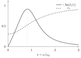
For $g=1.2$, the real-axis loss maximum lies at $x\simeq0.824$ although $\epsilon_1$ never crosses zero. The complex zero is $0.8-0.6i$: neither its real part nor a real-axis zero is an exact recipe for locating this broad loss maximum.

Dimensionality and electromagnetic boundaries

The bare kernel $e^2/(\epsilon_0Q^2)$ belongs to a three-dimensional bulk Fourier transform. Charges confined to a plane interact through their surrounding three-dimensional electric field and have a different in-plane kernel, which also changes in the presence of gates or dielectric interfaces. Replacing a bulk volume by a sheet area without changing the Coulomb problem gives incorrect screening and mode scales. Low-Dimensional Quantum Matter supplies the geometric context, and Plasmons develops material realizations.

A bulk dielectric zero is not a general surface-mode condition. Surface and interface modes satisfy boundary conditions on both sides; retarded polaritons also involve magnetic fields and propagation. Even the familiar quasistatic planar-interface condition involving the sum of two permittivities has assumptions about locality, isotropy and geometry. Finite films, anisotropic layers and nonlocal media require their own boundary problem. A reflectance edge or near-field resonance should therefore be compared with a model of the actual sample geometry.

A converged inversion answers the screening problem for the supplied $P$. Improving the basis, empty-band count and momentum grid cannot by itself repair missing electron–hole attraction or another error in that polarization approximation. Electronic Structure Methods Overview explains how these numerical and physical approximations differ.

Exercises

A microscopic field changes the macroscopic answer

For the two-component matrices in the text, calculate $\chi=P\epsilon^{-1}$ and verify $\epsilon^{-1}=I+v\chi$. Find the induced density and total field for $U_{\mathrm{ext}}=(1,0)^T$.

Solution

Direct multiplication gives

$$\chi=\begin{pmatrix}-7/22&-1/11\\-1/11&-5/11\end{pmatrix}.$$

Multiplying by $v$ on the left and adding the identity gives $\begin{pmatrix}4&-2\\-1&6\end{pmatrix}/11$, exactly the inverse dielectric matrix. The induced density is $(-7/22,-1/11)^T$, and

$$U_{\mathrm{tot}}=U_{\mathrm{ext}}+v\delta n =\frac1{11}\begin{pmatrix}4\\-1\end{pmatrix}.$$

The macroscopic ratio is $1/(4/11)=11/4$. The nonzero second component is the microscopic field that was lost when only $\epsilon_{00}$ was retained. Although the unsymmetrized $\epsilon$ is not symmetric, $\chi$ in this static reciprocal fixture is symmetric; matrix placement matters.

Why screening does not measure compressibility directly

Take the scalar static approximation $P=-\mathcal N$ with $\mathcal N>0$ and $v=e^2/(\epsilon_0Q^2)$. Compute $\chi$ and its small-$Q$ limit. Does a vanishing screened density response imply an incompressible reference?

Solution

$$\begin{aligned} \chi(Q,0)&=-\frac{\mathcal N}{1+v\mathcal N} =-\frac{\mathcal N Q^2}{Q^2+\kappa_{\mathrm{TF}}^2},\\ \chi(Q,0)&\sim-\frac{\epsilon_0Q^2}{e^2}=-\frac1v. \end{aligned}$$

The response to external potential energy vanishes because long-range Coulomb feedback suppresses net charge accumulation. The proper reference still has $\partial n/\partial\mu=\mathcal N>0$. A thermodynamic density change with the appropriate neutralizing background is different from applying a long-wavelength external electrostatic potential to a charged bulk.

Locate a loss maximum without a real dielectric zero

For $L(x)=gx/[(x^2-1)^2+g^2x^2]$ with $g=1.2$, determine the positive maximum and compare it with the complex zero $0.8-0.6i$ and the real-axis dielectric function.

Solution

The stationary condition is

$$3x^4+(g^2-2)x^2-1=0.$$

Only one root has $x^2>0$:

$$x_{\max}^2= \frac{2-g^2+\sqrt{(g^2-2)^2+12}}6.$$

Since $L$ vanishes at both zero and infinity and is positive between them, this stationary point is its maximum. It lies near $x=0.824$, rather than the real part $0.8$ of the complex zero. Meanwhile $\epsilon_1(x)>0$ for all positive real $x$. The damping is substantial; the broad maximum is compatible with a damped model response without providing a real-axis zero or a sharp long-lived excitation.

A background changes loss normalization

Suppose a calculation reports a background-normalized dielectric function $\bar\epsilon$ and the physical relative permittivity is $\epsilon_r=4\bar\epsilon$. Compare their zeros and loss functions. What changes if the background is frequency dependent and absorbing?

Solution

A nonzero real constant does not move the zeros, but

$$-\operatorname{Im}\epsilon_r^{-1} =\frac14\left[-\operatorname{Im}\bar\epsilon^{-1}\right].$$

Quoting the normalized loss as a physical loss would overstate its amplitude by four. If the background is complex and frequency dependent, use $\epsilon_r^{-1}=\epsilon_b^{-1}(\omega)\bar\epsilon^{-1}(\omega)$ before taking the imaginary part. The background can then alter peak shapes and add its own zeros or poles; neither a constant amplitude correction nor unchanged mode structure is generally justified.

References

• Adler, Stephen L. “Quantum Theory of the Dielectric Constant in Real Solids.” Physical Review 126, 413–420 (1962). doi:10.1103/PhysRev.126.413. Microscopic dielectric response, tensor structure and local-field corrections.
• GPAW developers. “Dielectric response: inverse dielectric function and symmetrized representation.” GPAW response-module documentation, accessed 14 October 2026. Explicit Coulomb factors in the microscopic response and macroscopic inverse-head construction.
• Onida, Giovanni, Lucia Reining, and Angel Rubio. “Electronic Excitations: Density-Functional versus Many-Body Green’s-Function Approaches.” Reviews of Modern Physics 74, 601–659 (2002). doi:10.1103/RevModPhys.74.601. Inverse dielectric response, macroscopic extraction, optical and loss spectra, and the distinction between local fields and polarization approximations.
• Wiser, Nathan. “Dielectric Constant with Local Field Effects Included.” Physical Review 129, 62–69 (1963). doi:10.1103/PhysRev.129.62. Self-consistent microscopic fields and the macroscopic longitudinal response.