Low-Dimensional Quantum Matter

A quantum system is low dimensional when its relevant low-energy degrees of freedom propagate in fewer than three spatial directions. The definition is operational: a thin sample is not automatically two dimensional, and an anisotropic three-dimensional crystal is not automatically a stack of independent planes. The occupied transverse modes, probe energy, scattering rate, correlation length, interaction range, and coupling to the environment all matter.

Reducing dimension changes more than geometry. It changes how states accumulate near a band edge, how long-wavelength fluctuations build up, which scattering processes are kinematically special, how screening works, whether disorder interference remains infrared finite, and which topological structures are possible. These effects make one- and two-dimensional systems unusually fertile, but they do not imply that every low-dimensional system is strongly correlated or lacks order.

Required background. Density of States supplies state counting and dimensional band-edge laws. Finite-Temperature Phase Transitions supplies the thermodynamic-limit and fluctuation criteria for a sharp phase transition. What Is Mesoscopic Physics? supplies the comparisons between confinement, coherence and sample size used to identify an effective dimension.

Reduced dimensionality and quantum fluctuations

We will follow three steps: identify the modes that remain active, count their states, and ask whether fluctuations destroy a proposed order. For a concrete device, use Quantum Wells, Quantum Wires or Quantum Dots for the confinement model. Here the emphasis is on the physical ideas shared by these systems.

Why Dimension Matters

Dimension controls the phase space available to particles and collective modes. For an isotropic momentum shell of radius $k$, the number of states scales as $k^{d-1}dk$. For a long-wavelength mode with stiffness proportional to $q^2$, the fluctuation weight contains $d^dq/q^2$. The same integer $d$ therefore enters state counting and long-distance stability in different ways.

Three broad changes recur:

• threshold structure: parabolic one-dimensional bands have inverse-square-root edge singularities, two-dimensional bands have steps, and three-dimensional bands turn on as a square root;
• infrared sensitivity: long-wavelength thermal fluctuations become progressively harder to suppress as $d$ decreases;
• kinematic restriction: conservation laws leave fewer independent scattering configurations, making special momenta such as $2k_F$ in one dimension unusually important.

Dimension also changes the mathematical objects available to phases. A two-dimensional gapped band can carry a Chern number and support a quantized Hall response. Two-dimensional configuration space permits anyonic exchange, while ordinary three-dimensional point particles have only bosonic or fermionic exchange classes. These are structural statements, not claims that topology appears in every two-dimensional material.

What Effective Dimension Means

Geometric and effective dimension

Let a sample have macroscopic lengths $L_x$, $L_y$, and $L_z$. Its geometric dimension describes which lengths are large compared with microscopic structure. Its effective quantum dimension describes which directions support occupied and resolvable low-energy motion.

If motion in one or more directions is confined, a single-particle spectrum can often be organized as

$$E_{n,\mathbf k_\parallel} = E_n^\perp + \varepsilon_\parallel(\mathbf k_\parallel),$$

where $n$ labels transverse modes and $\mathbf k_\parallel$ labels motion along unconfined directions. Define the first transverse gap

$$\Delta_\perp = E_1^\perp-E_0^\perp.$$

For noninteracting fermions at zero temperature, only the lowest subband is occupied when $E_0^\perp<\mu<E_1^\perp$. Write $E_F=\mu-E_0^\perp$. At nonzero temperature, the distance from the chemical potential to the next edge matters:

$$\delta_\perp=E_1^\perp-\mu=\Delta_\perp-E_F.$$

If $k_BT\ll\delta_\perp$, thermal occupation of that edge is exponentially suppressed. Spectral broadening and the reservoir energy window must also be small enough not to populate it. Requiring $E_F,k_BT,\Gamma,e|V|\ll\Delta_\perp$ is a convenient stronger condition, but $E_F\ll\Delta_\perp$ is not necessary at zero temperature. Here $\Gamma$ is an energy broadening and $V$ is the applied bias.

For dynamics, compare the probe energy with the allowed intersubband transitions. A photon whose energy lies above a gap does not automatically excite a discrete transition: its frequency, polarization and matrix element must match the transition. Interactions can also mix transverse modes virtually; a single-subband model requires that mixing to be small or incorporated into its effective parameters.

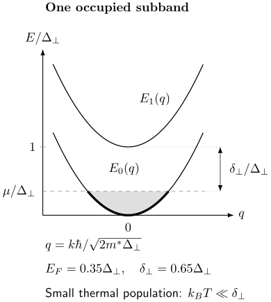
A cross-section of two subbands, $E_0(k)=\hbar^2k^2/(2m^\ast)$ and $E_1(k)=\Delta_\perp+E_0(k)$, with the lowest edge chosen as zero. The heavy arc marks occupied states at zero temperature. The illustrated $E_F=0.35\Delta_\perp$ leaves a clearance $\delta_\perp=0.65\Delta_\perp$ to the next edge. This clearance controls thermal population; the vertical intersubband transition at fixed momentum costs $\Delta_\perp$ in this ideal model.

Quasi-dimensional systems cross over

A layered tight-binding band illustrates a different route:

$$\varepsilon(\mathbf k) = \varepsilon_\parallel(k_x,k_y) -2t_\perp\cos(k_zc).$$

For $t_\perp=0$, the layers are kinematically independent. In an infinite stack within this metallic band model, nonzero coherent $t_\perp$ gives a dispersion in all three momenta, although a suitable intermediate regime can be approximately two dimensional. This statement assumes the coherent metal survives; an interaction-driven gap or localization can change its low-energy description. Whether interlayer motion is coherent also depends on broadening: the ratio $t_\perp/\Gamma$ is often as important as $t_\perp/k_BT$.

Critical behavior has its own crossover criterion. In a film with a fixed finite number of layers and short-range couplings, the longest-distance fluctuations are effectively two dimensional once the transverse correlation length reaches the thickness: the nonuniform transverse modes remain separated from the uniform mode. If the relevant symmetry permits a transition, its asymptotic film criticality need not be the bulk three-dimensional one. For an anisotropic film, compare the transverse correlation length with its physical thickness, or make the corresponding coordinate rescaling explicitly; an in-plane length alone is not that criterion. Radzihovsky’s finite-film scaling discussion separates this infrared limit from an intermediate bulk-like regime.

An infinite anisotropic stack is a different limit: sufficiently long-range correlations can resolve even weak nonzero interlayer coupling and recover three-dimensional critical behavior. Coupling finitely many isotropic short-range layers does not by itself evade the low-dimensional restrictions on continuous-symmetry breaking. “Two dimensional” must therefore name the observable, scale, and thermodynamic geometry.

Four dimensions that should not be conflated

Dimension	Meaning and useful measurements
Geometric	Macroscopically extended sample directions; determine them from thickness and structure.
Kinematic	Directions with active low-energy dispersion; examine subbands, Fermi-surface geometry and angular response.
Critical	Dimension of long-distance fluctuations near a transition; test finite-size and critical scaling.
Environmental	Space in which mediating fields and reservoirs propagate; examine dielectric, phonon, photon and substrate response.

A two-dimensional electron gas can interact through a three-dimensional Coulomb field. A monolayer can hybridize with three-dimensional substrate phonons. A one-dimensional edge channel can be attached to macroscopic reservoirs. These mixed-dimensional problems are common, not pathological.

Density of States by Dimension

Parabolic threshold law

For a quadratic minimum $E_{\mathbf k}=E_0+\hbar^2k^2/(2m^\ast)$, the number of states in a momentum shell is proportional to $k^{d-1}dk$. Since $dE/dk\propto k$, converting that shell to an energy interval gives

$$\nu_d(E)\propto k^{d-2} \propto(E-E_0)^{d/2-1}.$$

This relation applies above the edge, $E>E_0$. It explains the characteristic thresholds without memorizing three separate formulas:

Spatial dimension	Parabolic band edge
One	An integrable inverse-square-root divergence; many states lie close to the subband edge.
Two	A constant step; each new subband adds a constant density of states.
Three	A square-root onset; the density of states vanishes at the minimum.

The Density of States article gives the full state-counting derivation. Exercise 1 checks its prefactors and units. A quantum dot instead has discrete levels, $\nu_0(E)=\sum_j g_j\delta(E-E_j)$, with degeneracies $g_j$; finite lifetimes and measurement resolution broaden the peaks.

Dimension does not determine the DOS alone

The threshold law assumes a quadratic isotropic extremum. For a $d$-dimensional Dirac cone,

$$E_\pm(\mathbf k) = E_D\pm\hbar v|\mathbf k|,$$

the DOS instead scales as $\nu_d(E)\propto |E-E_D|^{d-1}$. Saddle points produce van Hove singularities, nearly flat bands concentrate states into narrow energy windows, and anisotropic masses change prefactors.

Thus a DOS feature can support a dimensional assignment only after the dispersion, degeneracy, broadening, and matrix elements are controlled. A sharp one-dimensional subband edge is not, by itself, evidence for strong interactions.

Enhanced Fluctuations

The infrared phase integral

The simplest diagnostic uses a continuous order parameter with slowly varying phase $\theta(\mathbf r)$ and stiffness $\rho_s$:

$$F[\theta] = \frac{\rho_s}{2} \int d^dx\,|\nabla\theta|^2.$$

Classical equipartition gives

$$\left\langle |\theta_{\mathbf q}|^2\right\rangle = \frac{k_BT}{\rho_s q^2}.$$

Writing $\Delta\theta(\mathbf r)=\theta(\mathbf r)-\theta(\mathbf 0)$, the relative phase variance contains

$$\begin{aligned} \left\langle [\Delta\theta(\mathbf r)]^2 \right\rangle &= \frac{2k_BT}{\rho_s} \mathcal I_d(\mathbf r), \\ \mathcal I_d(\mathbf r) &= \int\frac{d^dq}{(2\pi)^d} \frac{1-\cos(\mathbf q\cdot\mathbf r)}{q^2}. \end{aligned}$$

At large $r$ its infrared contribution behaves schematically as

$$\left\langle[\Delta\theta(r)]^2\right\rangle \sim \begin{cases} r, & d=1,\\ \ln(r/a), & d=2,\\ \text{finite}, & d>2, \end{cases}$$

where $a$ is a microscopic cutoff. The growth in one and two dimensions is the spin-wave intuition behind the restrictions proved by Hohenberg and by Mermin and Wagner. To see the connection to order, a Gaussian phase field gives

$$\langle e^{i[\theta(r)-\theta(0)]}\rangle =e^{-\langle[\Delta\theta(r)]^2\rangle/2}.$$

An unbounded phase variance makes this correlation tend to zero, so distant regions do not share a fixed phase. In two dimensions the logarithm produces a power law, with exponent $\eta=k_BT/(2\pi\rho_s)$ in this phase-only approximation.

What the no-order theorem does and does not say

For equilibrium systems with sufficiently short-range interactions, the thermodynamic limit, and an exact continuous symmetry, thermal fluctuations prevent conventional spontaneous long-range order in one and two dimensions under the theorem’s hypotheses. The statement has important boundaries:

• it concerns nonzero temperature, not every zero-temperature quantum ground state;
• it does not forbid finite-temperature breaking of a discrete symmetry, as the two-dimensional Ising model demonstrates;
• it does not forbid algebraic correlations or a Berezinskii–Kosterlitz–Thouless transition;
• magnetic anisotropy, explicit symmetry breaking, sufficiently long-range interactions, finite size, and coupling to an infinite stack can change the conclusion;
• a large but finite correlation length can look ordered on a finite sample or within a finite observation time.

Saying “two-dimensional magnets cannot order” without these qualifiers is incorrect. Real monolayer magnets can order because spin–orbit coupling supplies anisotropy and removes the exact isotropic continuous symmetry assumed by the simplest theorem.

BKT order and algebraic correlations

In an easy-plane or superfluid system, a vortex has the approximate energy and positional entropy

$$\begin{aligned} E_v &\simeq \pi\rho_s\ln\frac{L}{a}, \\ S_v &\simeq 2k_B\ln\frac{L}{a}. \end{aligned}$$

The single-vortex free-energy estimate changes sign when entropy can overcome stiffness. The full Berezinskii–Kosterlitz–Thouless theory treats interacting vortex pairs and renormalized stiffness; Nelson and Kosterlitz showed that it predicts the universal jump

$$\rho_s(T_{\mathrm{BKT}}^-) = \frac{2}{\pi}k_BT_{\mathrm{BKT}}$$

when $\rho_s$ is expressed in energy units. For the ideal neutral two-dimensional phase model at nonzero temperature below the transition, correlations decay algebraically rather than approaching a nonzero constant. In a charged superconducting film, electromagnetic screening introduces an additional length scale; applying the logarithmic-vortex picture requires the appropriate spatial regime. This is a distinct form of low-dimensional organization, not an exception that restores ordinary continuous-symmetry breaking.

Thermal and quantum dimensions differ

At a quantum critical point, imaginary time adds a scaling direction. If frequency scales as $\omega\sim q^z$, a common power-counting combination is

$$d_{\mathrm{eff}}^{\mathrm{critical}} = d+z.$$

This is a scaling relation, not permission to replace every $d$-dimensional quantum system by an isotropic classical system in $d+z$ dimensions. Conservation laws, long-range forces, damping, boundaries, and anisotropic scaling can alter the mapping. Quantum Criticality develops those qualifications.

Why Interactions Become More Consequential

Lower dimension does not automatically mean strong coupling

Interaction strength is always a ratio. Confinement can reduce kinetic phase space, weaken screening, or increase wave-function overlap, but a small interaction matrix element, large velocity, broad band, or strongly screening dielectric environment can still leave a controlled weak-coupling regime.

For a conventional two-dimensional electron gas with areal density $n$,

$$\begin{aligned} a&=\frac{1}{\sqrt{\pi n}},\\ a_B^\ast&=\frac{4\pi\epsilon\hbar^2}{m^\ast e^2},\\ r_s&=\frac{a}{a_B^\ast}. \end{aligned}$$

Here $\epsilon$ is the absolute permittivity in SI units. The ratio $r_s$ compares a typical Coulomb scale with the Fermi kinetic scale up to convention-dependent constants. Lowering $n$ increases $r_s\propto n^{-1/2}$. This density scaling is not universal: for an ideal two-dimensional Dirac cone, the analogous coupling

$$\alpha_{\mathrm{eff}} = \frac{e^2}{4\pi\epsilon\hbar v_F}$$

is density independent before velocity renormalization and environmental effects are included.

One-dimensional kinematics reorganizes the low-energy theory

A one-dimensional Fermi sea has two Fermi points rather than a Fermi surface of finite dimension. Particle–hole response is singular near $2k_F$, and repeated forward and backward scattering cannot generally be summarized by long-lived electron-like quasiparticles. Generic gapless interacting one-dimensional fluids instead organize into collective density modes with interaction-dependent power laws.

Haldane developed this collective description; Giamarchi gives a detailed treatment. This is the domain of the Luttinger-liquid description. It is powerful but not universal to every one-dimensional system: commensurability, disorder, spin gaps, confinement, long-range forces, or symmetry breaking can produce gapped or localized phases.

Confinement changes the interaction itself

Projecting a three-dimensional interaction into the lowest transverse mode gives a form-factor-dependent effective interaction,

$$V_{\mathrm{eff}}(\mathbf q_\parallel) = \int dz\,dz'\, |\phi_0(z)|^2 \times V(\mathbf q_\parallel;z,z') |\phi_0(z')|^2.$$

The layer thickness, gates, substrate dielectric function, nearby metallic screening, and higher subbands all enter. A bare $1/r$ law should not be inserted into a strictly lower-dimensional model without specifying this embedding.

Large DOS and strong correlation are different claims

A large DOS can amplify an interaction response, but does not identify a phase. Broadening can cut off a singularity, matrix elements can suppress a channel, and different orders can compete. What Are Strong Correlations? explains how to distinguish a DOS enhancement from quasiparticle failure, spectral-weight transfer and interaction-controlled scales.

Disorder, Topology, and Restricted Kinematics

Dimension also controls the return probability of a diffusing particle:

$$P(\mathbf 0,t) \propto (Dt)^{-d/2}.$$

The long-time interference correction involves $\int dt\,P(\mathbf0,t)$ and is increasingly infrared sensitive as $d$ decreases. This intuition underlies the special role of one and two dimensions in weak localization and one-parameter scaling. It does not mean every two-dimensional sample is experimentally insulating: finite dephasing, spin–orbit coupling, magnetic fields, topology, interactions, and symmetry class matter. The full statement belongs to Scaling Theory of Localization.

Restricted dimension can also stabilize responses with no direct three-dimensional analogue. The Integer Quantum Hall Effect uses a two-dimensional bulk and one-dimensional chiral boundary. The Fractional Quantum Hall Effect combines two-dimensional motion, magnetic flux, and interactions to produce fractionalized topological order. Dimensionality is necessary to these constructions but is not sufficient evidence for them.

Establishing Dimensionality

Compare a structural measurement with a measurement of the active modes. In a semiconductor well or wire, resolve subbands and their occupation. In an atomically thin crystal, compare layer count with electronic dispersion. In a layered bulk metal, look for momentum dependence perpendicular to the layers and changes with temperature or pressure. Cold-atom pancakes and tubes provide another realization, with a tunable transverse trap frequency.

Transport anisotropy alone does not establish reduced dimension: anisotropic masses or scattering times can make a three-dimensional metal conduct much better in one direction. Look for the crossover predicted by the proposed model, for example the onset of an additional subband as density increases. For collective behavior, also compare correlation lengths with the sample dimensions.

Worked estimate: a GaAs quantum well

Ando, Fowler and Stern review semiconductor subbands. As a simple estimate, take an infinite square well of width $L$ and effective mass $m^\ast$:

$$E_n^\perp = \frac{n^2\pi^2\hbar^2}{2m^\ast L^2}, \qquad n=1,2,\ldots$$

Taking $L=20\,\mathrm{nm}$ and $m^\ast=0.067m_e$ gives

$$\begin{aligned} E_1^\perp &\simeq 14\,\mathrm{meV}, \\ \Delta_\perp &= E_2^\perp-E_1^\perp \simeq 42\,\mathrm{meV}. \end{aligned}$$

If $E_F=8\,\mathrm{meV}$, the clearance to the second subband is about $34\,\mathrm{meV}$. At $T=20\,\mathrm K$, $k_BT\simeq1.7\,\mathrm{meV}$; a broadening $\Gamma=0.5\,\mathrm{meV}$ is also much smaller than the clearance. Equilibrium low-energy transport is then well described by the lowest subband within this independent-electron model.

A resonant electric field with a component perpendicular to the well can instead drive the $1\to2$ intersubband transition near $42\,\mathrm{meV}$: the opposite-parity wavefunctions give a nonzero dipole matrix element $\langle2|z|1\rangle$. A field polarized purely in the plane does not drive that dipole transition in an ideal separable well. Thus the same sample needs a two-subband description for this resonant response. Finite barriers, collective shifts and band nonparabolicity refine the numerical transition energy.

Common pitfalls

Using one dimension for every excitation. Electrons confined to a plane can still interact through three-dimensional electromagnetic fields and couple to substrate phonons. State which degrees of freedom and energy range the description covers.

Mistaking a finite sample for a thermodynamic phase. If the correlation length exceeds the device size, the device may look ordered even when the infinite system has no conventional long-range order. Temperature and size dependence help separate these cases.

Exercises

Exercise 1: derive the band-edge exponent

Starting from $\nu_d(E)=gV_d\int d^dk\,(2\pi)^{-d}\delta(E-E_{\mathbf k})$, derive the DOS for an isotropic parabolic minimum in $d=1,2,3$. Here $g$ is the total internal degeneracy and $V_d$ is the length, area or volume of the sample. Check the physical units in each case.

Solution

Use $d^dk=S_{d-1}k^{d-1}dk$ and

$$\begin{aligned} \delta(E-E_{\mathbf k}) &= \frac{m^\ast}{\hbar^2k_E} \delta(k-k_E), \\ k_E &= \frac{\sqrt{2m^\ast(E-E_0)}}{\hbar}. \end{aligned}$$

Then

$$\frac{\nu_d(E)}{V_d} = \frac{gS_{d-1}}{(2\pi)^d} \frac{m^\ast}{\hbar^2} k_E^{d-2}\Theta(E-E_0).$$

Substituting $S_0=2$, $S_1=2\pi$, and $S_2=4\pi$ gives

$$\begin{aligned} \nu_1/L&=\frac{g}{\pi\hbar}\sqrt{\frac{m^\ast}{2(E-E_0)}},\\ \nu_2/A&=\frac{gm^\ast}{2\pi\hbar^2},\\ \nu_3/V&=\frac{g}{4\pi^2} \left(\frac{2m^\ast}{\hbar^2}\right)^{3/2}\sqrt{E-E_0}, \end{aligned}$$

for $E>E_0$, and zero below the minimum. Because $V_d$ has units of length$^d$, $\nu_d/V_d$ has units of energy$^{-1}$ length$^{-d}$.

Exercise 2: second-subband threshold

For the GaAs well in the worked estimate, take spin degeneracy $g=2$. At what areal density does the zero-temperature in-plane Fermi energy reach $\Delta_\perp=42\,\mathrm{meV}$? Use the ideal two-dimensional parabolic gas.

Solution

For total degeneracy $g$,

$$n = \frac{gk_F^2}{4\pi}, \qquad E_F = \frac{\hbar^2k_F^2}{2m^\ast} = \frac{2\pi\hbar^2n}{gm^\ast}.$$

With $g=2$,

$$n_{\mathrm{th}} = \frac{m^\ast\Delta_\perp}{\pi\hbar^2} \simeq 1.18\times10^{12}\,\mathrm{cm}^{-2}.$$

Near this density the second subband begins to populate in the ideal model. Temperature, disorder, electrostatic self-consistency, and finite barriers smear or shift the threshold.

Exercise 3: infrared phase fluctuations

Use power counting to determine whether $\int_{q_{\mathrm{IR}}}^{\Lambda}d^dq/q^2$ diverges as $q_{\mathrm{IR}}\to0$ for $d=1,2,3$. Explain why this integral is only an intuition for, not a complete proof of, the no-order theorem.

Solution

Angular integration leaves

$$I_d \propto \int_{q_{\mathrm{IR}}}^{\Lambda} dq\,q^{d-3}.$$

Thus

$$\begin{aligned} I_1&\propto q_{\mathrm{IR}}^{-1},\\ I_2&\propto \ln(\Lambda/q_{\mathrm{IR}}),\\ I_3&\propto \Lambda-q_{\mathrm{IR}}. \end{aligned}$$

The first two are infrared divergent, while the third is finite. This Gaussian phase argument identifies the dangerous soft modes but does not establish all theorem hypotheses, control vortices, handle amplitude fluctuations, or cover long-range interactions and explicit anisotropy. The rigorous Hohenberg and Mermin–Wagner results use inequalities tied to the microscopic symmetry and interactions.

Exercise 4: vortex free energy

Using the vortex energy and entropy estimates, find the temperature at which the coefficient of $\ln(L/a)$ changes sign. Why is the result not yet the exact BKT transition criterion?

Solution

The free energy is

$$F_v \simeq \left(\pi\rho_s-2k_BT\right) \ln\frac{L}{a}.$$

The bare estimate changes sign at $k_BT=\pi\rho_s/2$. Near the transition, however, vortex–antivortex pairs screen each other and renormalize the stiffness. The exact universal statement uses the long-distance renormalized stiffness evaluated just below the transition,

$$\rho_s(T_{\mathrm{BKT}}^-) = \frac{2k_BT_{\mathrm{BKT}}}{\pi}.$$

The two formulas are consistent only after distinguishing bare from renormalized quantities.

Exercise 5: density and interaction strength

Show that $r_s\propto n^{-1/2}$ for a parabolic two-dimensional electron gas with fixed $m^\ast$ and dielectric constant. Why does the same argument not give a density-dependent coupling for an ideal Dirac cone?

Solution

The mean spacing scales as $a\sim n^{-1/2}$. The Coulomb energy scales as $E_C\sim e^2/(\epsilon a)\propto n^{1/2}$, while the parabolic Fermi energy scales as $E_F\propto k_F^2/m^\ast\propto n$. Therefore

$$\frac{E_C}{E_F} \propto n^{-1/2},$$

which is the scaling of $r_s=a/a_B^\ast$. For a Dirac cone, $E_F\sim\hbar v_Fk_F\propto n^{1/2}$, the same density scaling as $E_C$. Their ratio is therefore the approximately density-independent $\alpha_{\mathrm{eff}}$, subject to velocity renormalization, screening, and band-curvature corrections.

Exercise 6: test a dimensionality claim

A layered conductor has $\rho_c/\rho_{ab}=10^4$, and a paper calls it a two-dimensional metal. List three additional measurements or controls needed to make that claim convincing.

Solution

Resistivity anisotropy mixes band velocity and scattering-time anisotropy, so it is not sufficient. Useful independent checks include:

1. ARPES or quantum oscillations resolving negligible or finite $k_z$ dispersion;
2. angle-dependent magnetoresistance testing cylindrical versus warped three-dimensional orbits;
3. a temperature or pressure scan looking for coherent interlayer crossover;
4. optical conductivity comparing the interlayer bandwidth with $\Gamma$;
5. thickness dependence or subband structure in exfoliated samples.

The claim should also name the energy range: the same material may be quasi-two-dimensional above an interlayer coherence scale and three dimensional below it.

References

• T. Ando, A. B. Fowler, and F. Stern, “Electronic Properties of Two-Dimensional Systems,” Reviews of Modern Physics 54, 437–672 (1982), doi:10.1103/RevModPhys.54.437.
• T. Giamarchi, Quantum Physics in One Dimension (Oxford University Press, 2003), doi:10.1093/acprof:oso/9780198525004.001.0001.
• F. D. M. Haldane, “‘Luttinger liquid theory’ of one-dimensional quantum fluids. I. Properties of the Luttinger model and their extension to the general 1D interacting spinless Fermi gas,” Journal of Physics C: Solid State Physics 14, 2585–2609 (1981), doi:10.1088/0022-3719/14/19/010.
• P. C. Hohenberg, “Existence of Long-Range Order in One and Two Dimensions,” Physical Review 158, 383–386 (1967), doi:10.1103/PhysRev.158.383.
• D. R. Nelson and J. M. Kosterlitz, “Universal Jump in the Superfluid Density of Two-Dimensional Superfluids,” Physical Review Letters 39, 1201–1205 (1977), doi:10.1103/PhysRevLett.39.1201.
• L. Radzihovsky, “Lecture 5: The Renormalization Group,” Physics 7240: Advanced Statistical Mechanics, University of Colorado Boulder (8 November 2022), film scaling and Eq. (32), lecture notes.