van der Waals Heterostructures

A van der Waals heterostructure is an ordered stack of atomically thin crystals whose adjacent sheets are held together primarily by interlayer adhesion rather than by a three-dimensional network of covalent bonds. The weakly bonded interface relaxes the lattice-matching constraint of conventional epitaxy, allowing conductors, semiconductors, insulators, magnets, and superconductors to be combined with atomic-layer precision.

That freedom does not make the layers independent. Interlayer tunneling, charge transfer, dielectric screening, strain, phonons, exchange, and electrostatic fields can all cross the interface. Relative rotation and translation determine which momenta and orbitals communicate. Encapsulation, gates, spacers, and contacts are therefore part of the Hamiltonian, not merely packaging.

Required background. Two-Dimensional Materials supplies the constituent sheets and their dielectric environments. Band Theory Overview supplies band filling, hybridization and gap terminology. Quantum Wells supplies confinement subbands and heterointerface matching, needed to distinguish a stack’s geometry from its electronic states.

Stacked layers and interfacial electronic structure

A stack can change a layer’s behavior through several distinct mechanisms. We will distinguish direct electron tunneling from electrostatic coupling, then use that distinction to interpret avoided crossings, proximity effects and vertical current. Geim and Grigorieva (2013) introduce the broader materials approach; Graphene and Transition-Metal Dichalcogenides develop specific constituent layers.

A stack is a coupled quantum system

For two layers, a broad single-particle starting point is

$$\mathcal H = \begin{pmatrix} H_1+U_1 & T\\ T^\dagger & H_2+U_2 \end{pmatrix}.$$

$H_1$ and $H_2$ contain the isolated-layer bands in chosen bases. $U_1$ and $U_2$ include electrostatic offsets and any layer-local perturbations. The matrix $T$ carries interlayer tunneling, including orbital, spin, momentum, and position dependence. Coulomb interactions, lattice relaxation, disorder, and dynamical screening must be added when relevant.

This form separates three physically distinct statements:

• recognizable layers: eigenstates can still be associated mainly with one constituent;
• hybridized layers: $T$ transfers appreciable spectral weight between constituents;
• electrostatically coupled layers: $U_i$ and interactions change even if direct tunneling is weak.

The distinction matters experimentally. A shifted Raman or exciton line can result from strain, dielectric screening, doping, or hybridization. “The layers interact” is true in all four cases but does not identify the mechanism.

For one level in each layer,

$$H_2 = \begin{pmatrix} E_1 & t\\ t^* & E_2 \end{pmatrix},$$

with eigenvalues

$$E_\pm = \frac{E_1+E_2}{2} \pm \sqrt{ \left(\frac{E_1-E_2}{2}\right)^2 +|t|^2 }.$$

At resonance, $E_1=E_2$, the avoided-crossing gap is $2|t|$. Far from resonance, the energy shift is small and the states remain layer polarized. An avoided crossing with exchanged layer or optical character is therefore stronger evidence for coherent hybridization than two nearby peaks alone.

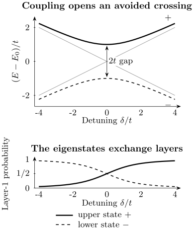
Calculated two-level example with constant real $t>0$, $E_0=(E_1+E_2)/2$ and detuning $\delta=E_1-E_2$. Top: the exact eigenenergies are separated by $2t$ at resonance; gray lines show the uncoupled energies. Bottom: each eigenstate changes its layer composition continuously through the crossing. At resonance both have equal layer weights. A measured change of character helps distinguish coherent mixing from unrelated nearby peaks. Exercise 1 derives the curves.

Band alignment is an interface property

Type-I, type-II, and type-III labels organize whether electron and hole band edges favor the same layer, opposite layers, or an overlapping broken-gap arrangement. They are useful starting points, not immutable properties of two isolated materials. The assembled interface can acquire a dipole, strain, charge transfer and dielectric self-energy shifts, while tunneling can create anticrossings. Thus tabulated isolated-material electron affinities need not give the operating band alignment. Photoemission and tunneling spectroscopy probe charged electronic states; an optical resonance also contains electron–hole binding. Compare quantities measured under compatible density, field and interface conditions.

Clean does not mean featureless

Dry pickup can keep polymer away from an internal interface, but it does not guarantee a uniform one. Hydrocarbons, adsorbed water, and air can aggregate into bubbles as the surrounding regions self-clean. Wrinkles, folds, tears, edge debris, trapped particles, and transfer-induced strain remain possible. Purdie and collaborators (2018) demonstrate how moving trapped contamination can recover clean regions. Cleaning can also change strain or damage sensitive layers, so the measured region still matters.

The physically active region must be located rather than assumed. Useful checks include optical and atomic-force microscopy, Raman strain and doping maps, photoluminescence maps, transmission electron microscopy where appropriate, scanning probes, and spatially resolved transport or microwave response. A high mobility averaged over one path does not prove that every interface region is uniform.

Rotation changes momentum matching

Rotation controls momentum communication

Let $\mathbf K_1$ and $\mathbf K_2$ denote corresponding crystal momenta in two layers. Relative rotation $\theta$ creates the mismatch

$$\Delta\mathbf K(\theta) = R(\theta)\mathbf K_2-\mathbf K_1.$$

For clean crystalline layers, a tunneling matrix element between Bloch states contains momentum-matching channels of the form

$$\mathbf k_1+\mathbf G_1 = \mathbf k_2+\mathbf G_2.$$

Here all vectors are expressed in the same laboratory frame, so the reciprocal vectors of the rotated layer are rotated too. A generic incommensurate bilayer need not possess an exact common translation lattice. This matching describes overlaps of the Bloch waves’ Fourier components. Twist can therefore suppress, enable, or resonantly tune tunneling between particular valleys and Fermi contours. Disorder, phonons, finite device size, and a moiré reciprocal lattice broaden or supplement the momentum-transfer channels. The observation of current does not by itself mean that bare in-plane momentum was conserved.

Relative translation also matters at atomic registry, and nonuniform strain makes the local angle and mismatch position dependent. For small-angle structures, lattice relaxation can produce large stacking domains separated by solitons. A single nominal twist number is then only the beginning of the structural description.

Alignment is measured, not inferred from a straight edge

Crystallographic edges can be armchair, zigzag, reconstructed, faceted, or unrelated to a visible cleavage line. Better alignment evidence may come from:

Probe	Information and limitation
Polarization-resolved second-harmonic generation	Crystal axes in suitable noncentrosymmetric layers; interference and layer symmetry affect the angular pattern.
Raman spectroscopy or diffraction	Stacking, strain or reciprocal-lattice orientation; the result averages over the illuminated region.
Scanning-probe moiré imaging	Local period and reconstruction; a small field of view need not describe the whole device.
Tunneling resonance	Alignment of the active electronic states; density, disorder, bias and contacts also affect the response.

An angle measured over a whole flake and a local angle can differ when strain or reconstruction varies across it. Mishchenko and collaborators (2014) used aligned graphene electrodes to observe momentum-sensitive resonant tunneling, illustrating an electronic consequence of orientation.

Encapsulation, electrostatics and contacts

Encapsulation is an active materials choice

Hexagonal boron nitride is widely used because it can provide an atomically flat, comparatively low-disorder dielectric and an excellent tunnel barrier. Dean and collaborators (2010) established its usefulness as a substrate for high-quality graphene. Its role depends on thickness and placement:

• as a substrate, it changes roughness, charge disorder, and screening;
• as a cap, it protects air-sensitive layers and modifies the top dielectric;
• as a spacer, it suppresses tunneling; electrostatic coupling can remain appreciable, while exchange generally also depends strongly on spacer thickness;
• as a gate dielectric, it sets capacitance and breakdown constraints;
• when crystallographically aligned, it can itself create a moiré perturbation.

It is therefore misleading to call hBN completely inert. Remote phonons, lattice alignment, dielectric screening, defects, trapped charge, and pressure all can affect the active layer. Other encapsulants have different chemical stability, permittivity, phonons and band offsets.

The stack determines which voltages are independent

A dual-gated drawing suggests separate control of total density and transverse displacement, but the actual map from voltages to layer densities is a capacitance problem. Geometric capacitances, quantum capacitance, contact potentials, screening by nearby graphite, trapped charge, and leakage all enter. In a multilayer device, each conducting sheet can have a distinct electrochemical potential.

Two-Dimensional Materials gives the canonical two-gate coordinate convention. In a more general stack, let $\phi_i$ be the electrostatic potential of conducting sheet $i$. In a network of geometric capacitances per area $c_{ij}=c_{ji}\ge0$, the sheet charge density is

$$Q_i=\sum_{j\ne i}c_{ij}(\phi_i-\phi_j).$$

The sum includes nearby sheets and gates; a gate connected to a voltage source has prescribed $\phi_j=V_j$. Grounded surroundings can be included as another node. The coefficients $c_{ij}$ are positive pair capacitances, whereas the corresponding Maxwell capacitance matrix has diagonal entries $\sum_j c_{ij}$ and off-diagonal entries $-c_{ij}$.

Close these equations with $Q_i=-en_i$ for excess electron density $n_i$ and the layer’s chemical potential $\mu_i(n_i)$. For a contacted sheet in equilibrium, $\mu_i(n_i)-e\phi_i$ equals its reservoir electrochemical potential; for a floating isolated sheet, its fixed total charge supplies the constraint. This is how finite compressibility enters. Treating every sheet as a perfect metal would discard that physics.

Good gate coordinates are verified experimentally. Charge neutrality, Landau filling, capacitance, compressibility, optical oscillator transfer, or a known commensurate density can provide anchors. Constant-density and constant-displacement sweeps should be stated in calibrated coordinates, not merely as diagonal lines on an arbitrary two-voltage plot.

Contacts define the open system

Top contacts can damage or dope an exposed surface; edge contacts can access an encapsulated conductor, as demonstrated by Wang and collaborators (2013); graphene contacts can be electrostatically tuned; tunnel contacts trade invasiveness for resistance. In semiconducting layers, Schottky barriers and contact-gate regions can dominate two-terminal behavior. In vertical devices, the electrodes are also part of the tunneling spectral function.

A device interpretation should separate channel, contact, and leakage contributions by using four-terminal measurements where possible, multiple contact pairs, length scaling, bias dependence, and gate-selective contact control. A resistance peak may belong to the channel, an injection barrier, a depleted lead, or a parallel path.

How a neighboring layer modifies the Hamiltonian

Integrating out a layer exposes the mechanism

For

$$\mathcal H = \begin{pmatrix} H_1 & T\\ T^\dagger & H_2 \end{pmatrix},$$

take this to be a quadratic single-particle block Hamiltonian, or a specified quadratic BdG model in a stated Nambu basis. For the retarded energy argument $z=E+i0^+$, block inversion gives

$$\begin{aligned} G_1^{-1}(z) &=z-H_1-\Sigma_1(z), \\ \Sigma_1(z) &=T(z-H_2)^{-1}T^\dagger. \end{aligned}$$

Read from right to left, this proximity self-energy sends a layer-1 state into layer 2 through $T^\dagger$, propagates it with the retarded resolvent $(z-H_2)^{-1}$, and returns it through $T$. The argument $E$ and each $H_i$ have energy units; an angular-frequency argument would instead enter as $\hbar\omega$.

The matrix structure of $\Sigma_1$ can induce spin–orbit terms, exchange fields, layer or sublattice masses, pairing amplitudes in Nambu space, and velocity changes. For a continuum parent or a specified broadening model its anti-Hermitian part also describes escape; an isolated finite Hermitian parent instead gives discrete hybridization poles. Arbitrary many-body self-energies and feedback on the parent are additional inputs, not consequences already contained in the bare block inversion. This formula describes hybridization-mediated proximity. It does not include every interfacial effect: static charge transfer, dielectric screening, remote Coulomb coupling, and strain can act even when coherent tunneling is negligible.

For two off-resonant levels with detuning $\Delta=E_1-E_2$,

$$\delta E_1 \simeq \frac{|t|^2}{\Delta}, \qquad w_2 \simeq \frac{|t|^2}{\Delta^2}.$$

The inherited energy scale and foreign-layer weight increase as detuning decreases. That gives a recurring tradeoff: stronger proximity often comes with more hybridization, scattering, or loss of the original layer identity. Large fitted proximity parameters should be checked against observed anticrossings, linewidths, and spectral-weight transfer.

Name the channel before naming the effect

Coupling	What can help distinguish it
Spin–orbit hybridization	Spin-lifetime anisotropy, band splitting and magnetoconductance analyzed in the appropriate scattering regime.
Magnetic exchange	Correlation with the source magnet’s domains and magnetization, plus spacer-thickness dependence.
Superconducting pairing	Andreev spectra, Josephson current and phase-dependent response.
Dielectric screening	Quasiparticle and optical shifts that change with the dielectric geometry even when tunneling is suppressed.
Charge transfer	Work-function, density and core-level shifts consistent with electrochemical equilibration.

For example, Ghiasi and collaborators (2017) measured spin-lifetime anisotropy in graphene/TMD structures. That probes spin dynamics directly and complements charge magnetoconductance. Disorder, stray fields, strain and parallel conduction can produce competing responses, so agreement among different probes matters.

Spin–Orbit Coupling in Solids develops spin Hamiltonians, and Exchange Interactions develops magnetic mechanisms. Superconducting Proximity Effect explains anomalous propagation through a stack; Proximity and Andreev Physics treats interface scattering and confined Andreev levels.

Vertical current probes spectral overlap

For weak tunneling between independently equilibrated electrodes at the same temperature, define $eV=\mu_1-\mu_2$ and let $E$ be measured from $\mu_1$. Write the isolated-electrode spectral matrices as $A_i(E)=-\operatorname{Im}G_i^R(E)/\pi$, with $\operatorname{Im}G=(G-G^\dagger)/(2i)$ and energy arguments measured from each electrode’s own chemical potential. For a complete canonical electron-channel basis, $\int dE\,A_i(E)=I$; the channel trace includes momentum, spin and orbital indices, without duplicated Nambu components or an extra spin-degeneracy factor. To leading order in $T$,

$$\begin{aligned} I(V) &=\frac{2\pi e}{\hbar}\int dE\,\mathcal T(E,V)[f(E)-f(E+eV)], \\ \mathcal T(E,V) &=\operatorname{Tr}\!\Bigl[T A_2(E+eV)T^\dagger A_1(E)\Bigr]. \end{aligned}$$

Here $I$ is $e$ times the net electron-number flow from electrode 1 to 2: for charge $-e$, this is the conventional charge current from 2 to 1. A positive small $\mu_1-\mu_2$ therefore gives positive $I$ under this direction convention. If both spin channels are identical and excluded from the explicit trace, their separate factor of two recovers the often-used $4\pi e/\hbar$ prefactor. In a basis with diagonal spectral matrices the trace is $\sum_{a,b}|T_{ab}|^2 A_{1,a}(E)A_{2,b}(E+eV)$.

The spectral functions include each isolated electrode’s band structure, lifetime, and interactions; the formula neglects higher-order tunneling and correlations between electrodes that require additional vertex or nonequilibrium dynamics. The matrix element contains barrier thickness, orbital overlap, twist, and momentum selection. Gates can tune density and relative alignment; bias changes the energy window. Resonant spectral overlap can produce a current peak and negative differential conductance, but series resistance, heating, charge trapping, and circuit instability must be excluded.

For a simple barrier estimate,

$$\kappa = \frac{\sqrt{2m_b(U-E)}}{\hbar}, \qquad \left|T(d)\right|^2 \propto e^{-2\kappa d}.$$

One extra atomic spacer can therefore change current by orders of magnitude. The formula is only a scaling guide: real hBN and semiconductor barriers have crystalline bands, momentum filtering, defects, image potentials, and bias-dependent profiles.

Exercises

Exercise 1: avoided crossing and layer character

For two layer-localized levels with $E_1=E_0+\delta/2$, $E_2=E_0-\delta/2$, and real tunneling $t$, find the eigenenergies. What gap appears at $\delta=0$, and what happens to layer character as $\delta$ changes sign?

Solution

Substitution into the two-level spectrum gives

$$E_\pm = E_0 \pm \sqrt{ \frac{\delta^2}{4}+t^2 }.$$

At resonance,

$$E_+-E_- = 2|t|.$$

For $|\delta|\gg|t|$, each eigenstate is localized mainly in one layer. Sweeping $\delta$ through zero continuously exchanges the dominant layer character between the two branches. For $t>0$, the normalized upper eigenvector has layer-1 probability

$$w_{1,+}=\frac12\left(1+\frac{\delta}{\sqrt{\delta^2+4t^2}}\right),$$

and $w_{1,-}=1-w_{1,+}$. This follows either by solving the two-component eigenvector equation or from $\partial E_+/\partial\delta=(w_{1,+}-w_{2,+})/2$. Both probabilities are $1/2$ at resonance. Their exchange is the lower panel of the figure.

Exercise 2: momentum matching under twist

Two clean layers have circular Fermi contours of radius $k_F$ whose centers differ by $\Delta K$. At a common chemical potential and zero temperature, ignoring reciprocal-lattice and phonon assistance, when are there momentum-matched states at the Fermi energy available for a small-bias tunneling conductance? What broadens the condition in a real device?

Solution

Elastic, momentum-conserving tunneling requires the two circles to intersect after one is displaced by $\Delta K$. Equal-radius circles intersect when

$$\Delta K\le 2k_F.$$

At $\Delta K=2k_F$ they touch at one point; for $0<\Delta K<2k_F$ they intersect at two points, and at $\Delta K=0$ the equal circles coincide. Finite lifetime, temperature, disorder, finite device size, phonons, moiré reciprocal vectors, and density inhomogeneity broaden or add momentum channels. At exactly zero bias the two directions balance and the net current is zero. The intersection condition concerns available states, not a guaranteed finite current: spin, orbital or other matrix-element selection rules may still suppress tunneling.

Exercise 3: one extra spacer layer

Suppose $\left|T(d)\right|^2\propto e^{-2\kappa d}$ with $\kappa=5.0\,\mathrm{nm}^{-1}$. Estimate the current ratio after adding $\Delta d=0.33\,\mathrm{nm}$ of an otherwise identical barrier.

Solution

At fixed spectral alignment, current scales with $\left|T\right|^2$, so

$$\begin{aligned} \frac{I(d+\Delta d)}{I(d)} &= e^{-2\kappa\Delta d} \\ &= e^{-3.30} \\ &\simeq 3.69\times10^{-2}. \end{aligned}$$

The simple model predicts a reduction by about a factor of $27$. A much weaker thickness dependence can signal defects, pinholes, inelastic channels, or a barrier model outside the WKB-like regime.

Exercise 4: dual-gate trajectories

Assume a contacted sheet in the large-positive-quantum-capacitance limit, with negligible trapping and leakage. Use $en=C_tV_t+C_bV_b$ and $2D=C_tV_t-C_bV_b$, with calibrated offsets suppressed and capacitances per area. If $C_t=0.20\,\mu\mathrm F/\mathrm{cm}^2$ and $C_b=0.10\,\mu\mathrm F/\mathrm{cm}^2$, find $dV_b/dV_t$ along constant density and constant displacement.

Solution

At constant density,

$$C_t\,dV_t+C_b\,dV_b=0,$$

so

$$\left. \frac{dV_b}{dV_t} \right|_n = -\frac{C_t}{C_b} = -2.$$

At constant displacement,

$$C_t\,dV_t-C_b\,dV_b=0,$$

and therefore

$$\left. \frac{dV_b}{dV_t} \right|_D = \frac{C_t}{C_b} = 2.$$

These are geometric-capacitance slopes. Quantum capacitance, trapped charge, or another conducting layer can curve or shift the experimental trajectories.

Exercise 5: off-resonant proximity scale

A layer-1 state couples to a remote layer-2 state with $|t|=20\,\mathrm{meV}$ and detuning $\Delta=0.40\,\mathrm{eV}$. Estimate the magnitude of the layer-1 energy shift and the layer-2 spectral weight.

Solution

Convert the detuning to $400\,\mathrm{meV}$. The shift magnitude is

$$\left|\delta E_1\right| \simeq \frac{(20\,\mathrm{meV})^2} {400\,\mathrm{meV}} = 1.0\,\mathrm{meV}.$$

The foreign-layer weight is approximately

$$w_2 \simeq \left( \frac{20}{400} \right)^2 = 2.5\times10^{-3}.$$

The sign of $\delta E_1$ follows the sign of $\Delta$. The estimate shows how a measurable induced scale can coexist with predominantly layer-1 character.

Exercise 6: interpreting a spin–orbit proximity signal

A graphene/TMD stack develops a broader weak-antilocalization cusp than a reference graphene device. The authors report proximity-induced spin–orbit coupling. List five checks needed before treating that mechanism as established.

Solution

Useful checks include:

1. fit the correct dimensional and intervalley-scattering regime rather than a generic one-parameter cusp;
2. measure temperature, density, and field-range dependence to separate dephasing and classical magnetoresistance;
3. compare covered and uncovered regions or devices with controlled interface thickness and cleanliness;
4. test spin transport or spin-lifetime anisotropy independently of charge magnetoconductance;
5. exclude parallel conduction, TMD contact effects, fringe fields, and charge-transfer disorder;
6. look for gate, twist, or spacer dependence predicted by the hybridization model.

Weak antilocalization is consistent with enhanced spin relaxation, but one curve does not uniquely determine the operator, magnitude, or interfacial origin of the coupling.

References

• C. R. Dean et al., “Boron Nitride Substrates for High-Quality Graphene Electronics,” Nature Nanotechnology 5, 722–726 (2010), doi:10.1038/nnano.2010.172.
• A. K. Geim and I. V. Grigorieva, “Van der Waals Heterostructures,” Nature 499, 419–425 (2013), doi:10.1038/nature12385.
• T. S. Ghiasi, J. Ingla-Aynés, A. A. Kaverzin, and B. J. van Wees, “Large Proximity-Induced Spin Lifetime Anisotropy in Transition-Metal Dichalcogenide/Graphene Heterostructures,” Nano Letters 17, 7528–7532 (2017), doi:10.1021/acs.nanolett.7b03460.
• A. Mishchenko et al., “Twist-Controlled Resonant Tunnelling in Graphene/Boron Nitride/Graphene Heterostructures,” Nature Nanotechnology 9, 808–813 (2014), doi:10.1038/nnano.2014.187.
• D. G. Purdie et al., “Cleaning Interfaces in Layered Materials Heterostructures,” Nature Communications 9, 5387 (2018), doi:10.1038/s41467-018-07558-3.
• L. Wang et al., “One-Dimensional Electrical Contact to a Two-Dimensional Material,” Science 342, 614–617 (2013), doi:10.1126/science.1244358.