Transition-Metal Dichalcogenides

A transition-metal dichalcogenide (TMD) has nominal composition $MX_2$ , with a transition metal $M$ between two chalcogen planes $X$ . That formula names a large materials family, not a single phase. Common group-VI monolayers such as MoS $_2$ , MoSe $_2$ , WS $_2$ , and WSe $_2$ are direct-gap semiconductors at the Brillouin-zone corners; compounds such as NbSe $_2$ and TaS $_2$ are metallic and can develop charge order or superconductivity; changes of polytype can produce still other band structures.

The semiconducting monolayers are especially instructive because several physical effects act together: broken inversion symmetry, strong atomic spin–orbit coupling, inequivalent $K$ and $K'$ valleys, large excitonic effects, and layer-sensitive band alignment. Stacking two layers adds registry, twist, lattice mismatch, relaxation, and electrostatic filling. The result is a platform whose simplest optical spectrum is already many-body physics and whose moiré descendants can realize narrow, interacting bands.

Required background. Two-Dimensional Materials supplies sheet screening and the distinction between layer structure and electronic dimension. Band Theory Overview supplies band extrema, gaps and filling. Spin–Orbit Coupling in Solids supplies the symmetry and energy-scale reasoning behind coupled spin, orbital and valley states.

Layered dichalcogenides and coupled degrees of freedom

We will use semiconducting group-VI monolayers to connect crystal symmetry to spin, valley and optical response, then follow those ingredients into a bilayer. Metallic compounds such as NbSe $_2$ and TaS $_2$ start from different bands; their ordering is discussed in Charge and Spin Density Waves and the superconductivity chapter.

Crystal structure and valley bands

The formula does not determine the Hamiltonian

Each monolayer contains an $X$ – $M$ – $X$ sandwich, but the local coordination can differ:

Structure	What it means for the low-energy model
1H	Trigonal-prismatic coordination; common group-VI sheets are semiconducting. A sheet exfoliated from 2H bulk is locally 1H.
1T	Octahedral coordination; often metallic and susceptible to reconstruction.
1T′	Distorted octahedral structure; anisotropic or inverted bands need a different model from the 1H valleys.
2H bulk	A two-layer hexagonal repeat; stacking can restore inversion, and the fundamental gap can become indirect.

The prefix counts the crystallographic repeat and the letter identifies stacking or coordination. Calling an isolated trigonal-prismatic sheet “2H monolayer” communicates its parent crystal but can obscure its actual one-layer symmetry. State both facts when the distinction matters.

An ideal 1H monolayer has point group $D_{3h}$ and lacks inversion. Its horizontal mirror plane constrains spin components, while threefold rotation organizes the valley optical matrix elements. A centrosymmetric 2H bilayer can recover spin degeneracy even though each constituent layer remains locally noncentrosymmetric. An electric displacement field, asymmetric dielectric environment, or different top and bottom layers can remove that restoration.

Valley ordering is material and thickness dependent

For common semiconducting group-VI monolayers, the lowest direct optical transitions occur near $K$ and $K'$ . The valence edge there is dominated by metal $d_{x^2-y^2}$ and $d_{xy}$ combinations, while the conduction edge has substantial $d_{z^2}$ character. This orbital content explains why spin–orbit splitting is generally much larger in the valence sector than in the simplest conduction sector.

The statement “a TMD monolayer has a direct gap” is not a theorem for every $MX_2$ . Even within the familiar compounds, nearby extrema at $\Gamma$ and the six $Q$ valleys affect transport, high doping, strain response, and multilayer crossover. Layer number changes hybridization differently at $K$ , $\Gamma$ , and $Q$ , and can move the fundamental gap away from the optically bright valley. A calculation or experiment should therefore report both the momentum of each edge and whether the quoted gap is quasiparticle, optical, or a density-dependent transport scale.

Monolayer Valley Hamiltonian

A two-band model fixes the leading convention

Let $\tau=\pm1$ label $K$ and $K'$ , let $s=\pm1$ denote the approximately out-of-plane spin, and let $\mathbf q$ be the wavevector measured from the chosen valley, with crystal-momentum offset $\hbar\mathbf q$ . In a basis of conduction- and valence-edge orbitals, the model of Xiao and collaborators (2012) is

H_{\tau s}(\mathbf q) = at\left( \tau q_x\sigma_x+q_y\sigma_y \right) +\frac{\Delta}{2}\sigma_z -\lambda\tau s \frac{\sigma_z-\mathbb I}{2}.

Here $a$ is a lattice-length convention, $t$ controls interband velocity, $\Delta$ is the gap parameter before the displayed spin splitting, and we choose $\lambda>0$ so that $2\lambda$ is the valence-edge splitting. Assume $\Delta>\lambda$ to keep the conduction and valence basis states in their stated order at both valleys. The Pauli matrices act in the two-orbital band-edge basis, not on real spin.

The eigenvalues are

\begin{aligned} E_{\tau s}^{\pm}(\mathbf q) &= \frac{\lambda\tau s}{2} \pm \sqrt{ a^2t^2q^2 + \frac{(\Delta-\lambda\tau s)^2}{4} }. \end{aligned}

At $\mathbf q=0$ ,

\begin{aligned} E_c(\tau,s)&=\frac{\Delta}{2},\\ E_v(\tau,s)&=-\frac{\Delta}{2}+\lambda\tau s. \end{aligned}

Thus the model gives a spin-independent conduction edge and a valence splitting $2\lambda$ at fixed valley. Real materials have a finite, material-dependent conduction splitting generated by remote bands and additional spin–orbit terms. Quantitative models may also need electron–hole asymmetry, trigonal warping, $Q$ valleys, strain, dielectric self-energy, and multiple orbitals. Kormányos and collaborators (2015) develop more detailed models. The two-band Hamiltonian is a useful starting point near $K$ and $K'$ , with $atq$ small enough that omitted bands remain far away.

Time reversal locks spin to valley without polarizing equilibrium

Time reversal reverses momentum and spin. With the above local valley coordinates,

E_{\tau s}(\mathbf q) = E_{-\tau,-s}(-\mathbf q).

The upper valence state at $K$ therefore has the opposite spin to its degenerate partner at $K'$ . This is spin–valley locking. For holes confined to the upper valence branches, a spin-conserving elastic perturbation cannot simply scatter between these partners: the target has the opposite spin. Other bands, spin mixing and inelastic processes limit this protection. In a time-reversal-invariant equilibrium state the partners are equally occupied, so spin–valley locking alone creates no net spin or valley polarization.

Circularly polarized light can address opposite valleys near the band edge. In one common convention, $\sigma^+$ couples most strongly at one valley and $\sigma^-$ at the other; reversing the valley or helicity convention swaps those labels. The invariant statement is about the dipole matrix elements,

P_\pm^{cv}(\mathbf q) = \frac{1}{\sqrt2} \left\langle u_{c\mathbf q} \middle| \hat v_x\pm i\hat v_y \middle| u_{v\mathbf q} \right\rangle ,

and their valley contrast. A helicity-resolved peak demonstrates a selection-rule-weighted optical response, not by itself a long-lived population, a dc valley current, or a topological invariant.

What optical lines reveal about spin and valley

A and B transitions are not a bare spin–orbit meter

The large valence splitting creates two prominent direct exciton families. The A exciton is built mainly from the upper spin-split valence band and the relevant conduction edge; the B exciton begins from the lower valence band. Schematically,

\begin{aligned} E_A^{\mathrm{opt}} &= E_{g,A}^{\mathrm{QP}}-E_{b,A}, \\ E_B^{\mathrm{opt}} &= E_{g,B}^{\mathrm{QP}}-E_{b,B}. \end{aligned}

Their separation is therefore

E_B^{\mathrm{opt}}-E_A^{\mathrm{opt}} = E_{g,B}^{\mathrm{QP}}-E_{g,A}^{\mathrm{QP}} - \left( E_{b,B}-E_{b,A} \right).

It is related to valence spin–orbit splitting, but it need not equal the bare splitting. Conduction-band spin structure, different reduced masses, exchange, screening, and band-dependent self-energy corrections all contribute. Extracting an atomic spin–orbit constant from the A–B peak spacing alone is therefore overconfident.

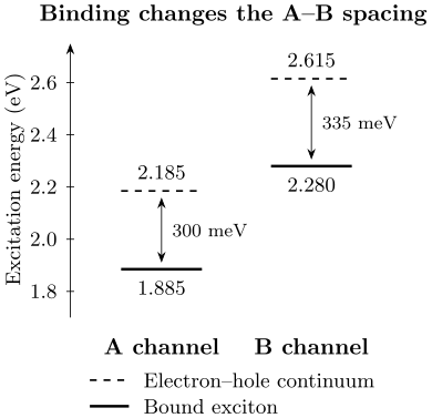
Two excitation channels have different continuum thresholds and binding energies; the optical A–B separation is smaller than the continuum separation. — An illustrative calculation, not a fit to a particular compound. Dashed lines are the A and B electron–hole continuum thresholds; solid lines are the bound excitons. With $\Delta=2.400\,\mathrm{eV}$ and $\lambda=0.215\,\mathrm{eV}$ in the minimal model, the thresholds differ by $430\,\mathrm{meV}$ . Binding energies of $300$ and $335\,\mathrm{meV}$ reduce the optical separation to $395\,\mathrm{meV}$ , as in Exercise 3. Both channels use the same many-electron ground-state energy as zero; the displayed axis omits lower energies.

The sign of the small conduction splitting controls whether the lowest intravalley exciton is spin-allowed or spin-forbidden. Tungsten-based and molybdenum-based compounds often have different bright–dark orderings, but the rule is not universal across dielectric environments, strain, density, layer configuration, and momentum-indirect states. State the compound and the ordering actually inferred.

Magnetic shifts combine several moments

For a specified exciton branch, a small out-of-plane field is often summarized by

\Delta E_X = g_X\mu_B B_z,

where the sign depends on how the two helicities or valleys are subtracted. The effective $g_X$ combines electron and hole spin and orbital magnetic moments. The division into atomic and intercellular orbital terms depends on the band model; Berry-curvature and effective-mass descriptions must not be added as if they were automatically independent corrections. It may also vary with exciton character, hybridization, and moiré registry.

For example, define $\Delta E_X=E_{\sigma^+}-E_{\sigma^-}$ before interpreting the sign of $g_X$ . A value near $-4$ does not identify a branch without its polarization and field dependence. Diamagnetic shifts, field-induced brightening, and exchange with resident carriers can enter beyond the simplest linear regime.

Bright, dark and interlayer excitons

Coulomb physics dominates the optical threshold

Reduced screening makes neutral electron–hole pairs prominent in monolayer spectra. The generic relation

E_{\mathrm{opt}} = E_g^{\mathrm{QP}}-E_b

is developed, together with nonlocal screening, on Two-Dimensional Materials. Here $E_g^{\mathrm{QP}}$ must be the continuum threshold in the same spin, valley and total-momentum channel as the bound state. A lower indirect continuum in a different channel cannot be subtracted indiscriminately. The exciton binding and nonlocal screening calculations of Berkelbach, Hybertsen and Reichman (2013) illustrate this distinction.

Excitation	Meaning and useful probe
A or B exciton	Different spin-split valence bands contribute to absorption or reflectance. Their spacing includes binding-energy differences.
Spin-dark exciton	An intravalley pair has a suppressed spin-allowed dipole; magnetic brightening can help reveal it.
Momentum-indirect exciton	The electron and hole occupy different momenta; emission generally needs a phonon, disorder or another momentum source.
Trion or exciton polaron	Resident charge modifies the optical excitation. Density-dependent spectra distinguish a dilute few-body picture from dressing by a Fermi sea.
Interlayer exciton	Electron and hole mainly occupy different layers; a Stark shift and layer-dependent excitation help establish this assignment.

Photoluminescence intensity depends on preparation, relaxation, light-cone occupation, nonradiative loss, collection, and matrix element. It is neither a direct population meter nor a binding-energy measurement. A neutral-exciton binding energy requires a quasiparticle gap from an independent or jointly constrained probe, not merely the separation between a PL peak and an assumed band edge.

At finite carrier density, an optical excitation interacts with a Fermi sea. The attractive and repulsive exciton-polaron branches can be more faithful than an isolated three-particle trion picture. Sidler and collaborators (2017) observed the transfer of oscillator strength between such resonances in charge-tunable MoSe₂. The useful description depends on density, Fermi energy and the observable.

Interlayer separation produces an electric dipole

In a type-II heterobilayer, the conduction and valence edges can favor different layers. An electron and hole then form an interlayer exciton with an out-of-plane electric dipole. To leading order, a local electric field produces

\Delta E_{\mathrm{IX}} \simeq -p_z E_z, \qquad p_z\simeq ed_{\mathrm{eff}},

Choose $+z$ from the electron layer toward the hole layer, so $p_z>0$ ; reversing that ordering reverses the dipole. The field $E_z$ is the local electric field, not the displacement field $D_z$ . The effective separation $d_{\mathrm{eff}}$ need not equal the geometric layer spacing. Interlayer separation can lengthen radiative lifetime, but hybridization, momentum mismatch, moiré localization, defects, and nonradiative channels also matter.

Rivera and collaborators (2015) combined resonant excitation, gate-dependent energy shifts and lifetime measurements to identify interlayer excitons in MoSe₂–WSe₂. Long lifetime alone is insufficient because dark intralayer states and traps can also emit slowly.

From a bilayer to moiré bands

Mismatch and twist set a long geometric scale

Near parallel or antiparallel alignment, often called R-type and H-type stacking respectively, the local atomic registry varies slowly across a bilayer. Moiré Superlattices derives the generic period and triangular-cell area from lattice mismatch and twist. Applied to a TMD pair, that construction must use the measured lattice constants, local angle, and heterostrain rather than a nominal fabrication angle.

For small mismatch $\delta=(a_2-a_1)/a_1$ and small angular deviation $\theta$ in radians from the chosen alignment, $L_M\simeq a_1/\sqrt{\delta^2+\theta^2}$ and $A_M=\sqrt3L_M^2/2$ . These leading-order expressions neglect strain and relaxation. Exercise 4 applies them.

The density $n_M=1/A_M$ represents one particle per measured moiré cell. Converting a gate voltage into filling $\nu=n/n_M$ still requires geometric capacitance, quantum capacitance, trapped charge, contact behavior, and any parallel conducting channels.

The moiré modulation of a carrier valley can be organized as

V_\tau(\mathbf r) = \sum_{j=1}^{3} \left[ V_j e^{i\mathbf G_j\cdot\mathbf r} + V_j^*e^{-i\mathbf G_j\cdot\mathbf r} \right],

where the shortest moiré reciprocal vectors $\mathbf G_j$ are related by threefold rotation. Depending on material and stacking, the continuum Hamiltonian also needs layer-dependent dispersions, interlayer tunnelling, displacement-field offsets, spin–valley structure, and lattice relaxation.

For an exciton center of mass $\mathbf R$ , a useful first reduction is

H_X = - \frac{\hbar^2\nabla_{\mathbf R}^2}{2M_X} +V_X(\mathbf R) +H_{\mathrm{valley}} +H_{\mathrm{exchange}}.

Here $M_X$ is the exciton center-of-mass mass, and $V_X$ is inherited from the registry dependence of band edges, binding, and hybridization. Multiple moiré exciton peaks can arise from quantized confinement, minibands, or hybridized intra- and interlayer excitons. Similar peak multiplicity can also come from strain, domains, phonon replicas, charged complexes, or disorder. Twist-angle dependence, spatial maps, polarization, density, temperature, and power dependence are therefore part of the identification.

TMD narrow bands do not require a graphene magic-angle mechanism

In twisted graphene, velocity renormalization of coupled Dirac cones motivates a special dimensionless coupling and magic-angle language. TMD band edges are often massive, and their moiré potentials can be strongly registry dependent. Large effective mass, long moiré period, and local band-edge modulation can make the kinetic bandwidth small without tuning to a graphene-like velocity zero.

That distinction does not make the problem simple. Atomic relaxation can reconstruct the nominal sinusoidal pattern into stacking domains and solitons. Heterostrain changes local periods and symmetries. Remote valleys can approach the active band. A displacement field can change layer polarization and bandwidth. A faithful model must show that the retained bands are isolated over the parameter window and that its Wannier or continuum representation preserves their symmetry and topology.

Interactions in a narrow moiré band

When a Hubbard description is useful

When a narrow, isolated moiré band admits localized orbitals, a common starting point is the generalized Hubbard model studied by Wu and collaborators (2018):

\begin{aligned} H &= H_t + U\sum_i n_{i+}n_{i-} +\frac{1}{2}\sum_{i\ne j}V_{ij}n_i n_j +H_{\mathrm{exchange}} +H_{\mathrm{remote}}, \\ H_t &= -\sum_{\langle ij\rangle,\alpha} t_{ij}^{\alpha} c_{i\alpha}^\dagger c_{j\alpha} +\mathrm{h.c.} \end{aligned}

Here $\alpha=+,-$ labels two retained flavors, often a time-reversed spin–valley pair, and $n_i=n_{i+}+n_{i-}$ . The interaction $U$ penalizes occupying both flavors on one site. Additional active layers or orbitals generally require more terms; the labels should not automatically be read as bare spin. The effective lattice can be triangular, honeycomb, or multi-orbital depending on stacking and which valley manifold is active. Complex hopping phases and Berry curvature can obstruct a naive one-orbital description or require a model that retains the band topology.

The useful hierarchy is not merely “ $U$ is large.” Compare

\begin{gathered} W,\quad U,\quad V_1,\quad \Delta_{\mathrm{remote}}, \\ k_BT,\quad \Gamma_{\mathrm{dis}},\quad E_Z,\quad E_{\mathrm{field}}. \end{gathered}

where $W$ is active-band width, $V_1$ a representative nonlocal interaction, $\Delta_{\mathrm{remote}}$ the gap to omitted bands, and $\Gamma_{\mathrm{dis}}$ a disorder scale. The hierarchy $W,U,V_1\ll\Delta_{\mathrm{remote}}$ is a useful sufficient starting point for perturbative band projection, provided the interaction matrix elements that mix bands are also small. It is not a universal necessary criterion: large diagonal repulsion alone does not determine interband mixing. If the separation fails, a one-band model needs an additional justification or a multiband treatment. Strong coupling requires interactions large relative to $W$ , while observing coherent low-energy order additionally requires temperature and inhomogeneity below the relevant collective scale.

Integer and fractional filling can favor different states

Insulation near one carrier per moiré cell can be consistent with Mott localization, but band gaps, flavor polarization, charge transfer, disorder, and symmetry breaking can also suppress transport. At fractional filling, longer-range repulsion can stabilize generalized Wigner crystals or other charge-ordered states. The commensurate filling is evidence for a moiré origin, not a complete phase diagnosis.

A resistance peak can arise from poor contacts or localization without a thermodynamic gap. Compressibility helps distinguish that case from an incompressible state; spatial or symmetry-sensitive measurements help identify charge order. Optical sensing detects how an exciton responds to resident carriers, so an exciton-energy anomaly is an indirect probe of those carriers, not an image of their arrangement. Regan and collaborators (2020) reported Mott and generalized Wigner-crystal states in WSe₂/WS₂; Exercise 6 asks which measurements distinguish the interpretations. See Correlated Insulators in Moiré Systems for the detailed comparison.

Superconductivity and the open pairing question

Xia and collaborators (2025) and Guo and collaborators (2025) reported superconductivity in twisted bilayer WSe₂, using zero-resistance regions together with current and magnetic-field dependence. These observations establish a phase to explain; they do not by themselves determine the pairing interaction or gap symmetry. The relation among correlations, phonons, band geometry and spin–valley structure remains an open microscopic question.

Moiré Superconductivity explains the relevant physical tests and models. Moiré Quantum Systems follows dated results and open questions. Intrinsic superconductivity in metallic NbSe₂ begins from a different band structure and should not be identified with this doped semiconducting bilayer.

Exercises

Exercise 1: band-edge splitting in the minimal model

Set $\mathbf q=0$ in the two-band Hamiltonian. Find the conduction and valence energies and show that the valence splitting at fixed $\tau$ is $2\lambda$ . Why does this not predict the full experimental A–B exciton separation?

Solution

At $\mathbf q=0$ , the conduction basis state has $\sigma_z=+1$ , so the spin–orbit projector $(\sigma_z-\mathbb I)/2$ vanishes:

E_c(\tau,s)=\frac{\Delta}{2}.

The valence basis state has $\sigma_z=-1$ , giving

E_v(\tau,s) = -\frac{\Delta}{2} + \lambda\tau s.

At fixed valley, changing $s$ from $+1$ to $-1$ changes the valence energy by magnitude

\left| E_v(\tau,+1)-E_v(\tau,-1) \right| = 2|\lambda|.

The A and B optical lines are excitons, not bare interband gaps. Their separation also contains conduction splitting, branch-dependent binding, exchange, effective masses, and quasiparticle self-energy corrections. Therefore it need not equal $2|\lambda|$ .

Exercise 2: time reversal and spin–valley locking

For the displayed spectrum, verify $E_{\tau s}(\mathbf q)=E_{-\tau,-s}(-\mathbf q)$ . Explain why spin–valley locking does not imply equilibrium magnetization.

Solution

The spectrum depends on $q^2$ and on the product $\tau s$ . Under

(\tau,s,\mathbf q) \longmapsto (-\tau,-s,-\mathbf q),

both $q^2$ and $\tau s$ remain unchanged, so the energies agree. The highest valence state at one valley is paired with an opposite-spin state at the other valley.

In equilibrium with time-reversal symmetry, the two partners have equal energy and equal statistical occupation. Their spin and orbital moments cancel when summed over valleys. A net magnetization requires unequal occupation or spontaneous time-reversal breaking, not merely spin–valley correlation.

Exercise 3: why the A–B spacing is not a bare constant

Let the two quasiparticle gaps be $E_{g,B}^{\mathrm{QP}}=E_{g,A}^{\mathrm{QP}}+\Delta_v$ and the two binding energies differ by $\delta E_b=E_{b,B}-E_{b,A}$ . Express the optical A–B separation. Evaluate it for $\Delta_v=430\,\mathrm{meV}$ and $\delta E_b=35\,\mathrm{meV}$ .

Solution

Using $E_j^{\mathrm{opt}}=E_{g,j}^{\mathrm{QP}}-E_{b,j}$ ,

\begin{aligned} E_B^{\mathrm{opt}}-E_A^{\mathrm{opt}} &= \Delta_v-\delta E_b\\ &= 430\,\mathrm{meV}-35\,\mathrm{meV}\\ &= 395\,\mathrm{meV}. \end{aligned}

Even in this simplified example, the optical separation differs from the quasiparticle valence contribution by $35\,\mathrm{meV}$ . Additional conduction, exchange, and self-energy terms can alter it further.

Exercise 4: moiré period and one-particle density

Take $a=0.33\,\mathrm{nm}$ , lattice mismatch $\delta=0.040$ , and twist $\theta=1.0^\circ$ . Estimate $L_M$ , $A_M$ , and the density for one particle per moiré cell.

Solution

First convert the angle to radians:

\theta = \frac{\pi}{180} \simeq 0.01745.

Then

\begin{aligned} L_M &\simeq \frac{0.33\,\mathrm{nm}} {\sqrt{0.040^2+0.01745^2}}\\ &\simeq 7.56\,\mathrm{nm}. \end{aligned}

The triangular-cell area is

\begin{aligned} A_M &= \frac{\sqrt3}{2}L_M^2\\ &\simeq 49.5\,\mathrm{nm}^2. \end{aligned}

Since $1\,\mathrm{nm}^{-2}=10^{14}\,\mathrm{cm}^{-2}$ ,

n_M = \frac{1}{A_M} \simeq 2.02\times10^{12}\,\mathrm{cm}^{-2}.

This is a geometric estimate. A voltage-to-filling conversion still needs a device capacitance and offset calibration.

Exercise 5: valley Zeeman scale

An exciton branch has $g_X=-4.0$ under the convention $\Delta E_X=E_{\sigma^+}-E_{\sigma^-}=g_X\mu_BB$ . Estimate the signed splitting at $B=9.0\,\mathrm T$ using $\mu_B=57.9\,\mu\mathrm{eV/T}$ .

Solution

\begin{aligned} \Delta E_X &= (-4.0) (57.9\,\mu\mathrm{eV/T}) (9.0\,\mathrm T)\\ &= -2084\,\mu\mathrm{eV}\\ &\simeq -2.08\,\mathrm{meV}. \end{aligned}

The magnitude is $2.08\,\mathrm{meV}$ . The minus sign says that $E_{\sigma^+}<E_{\sigma^-}$ under the stated subtraction convention; changing the helicity convention would change the reported sign.

Exercise 6: identifying a fractional-filling insulator

A WSe $_2$ /WS $_2$ device shows a resistance maximum and an exciton-energy kink at a gate voltage assigned to $\nu=1/3$ . The authors call the state a generalized Wigner crystal. List four checks that would materially strengthen or weaken that interpretation.

Solution

Useful checks include:

independently calibrate density and moiré-cell area, including trapped charge and spatial twist variation;
measure compressibility or capacitance to test thermodynamic incompressibility rather than contact-limited resistance;
map nearby rational fillings and temperature scales to test a systematic commensurability sequence;
use a spatial or symmetry-sensitive probe to seek the predicted charge pattern or broken lattice symmetry;
vary displacement field and dielectric screening to test the expected balance of $V_1/W$ ;
rule out ordinary localization, traps, parallel channels, and an accidental single-particle minigap.

The two anomalies are consistent with a filling-dependent state, assuming the filling assignment is correct. Repeating them across sweeps and devices tests reproducibility; neither anomaly alone determines a microscopic charge pattern.

References

T. C. Berkelbach, M. S. Hybertsen, and D. R. Reichman, “Theory of Neutral and Charged Excitons in Monolayer Transition Metal Dichalcogenides,” Physical Review B 88, 045318 (2013), doi:10.1103/PhysRevB.88.045318.
Y. Guo et al., “Superconductivity in 5.0° Twisted Bilayer WSe $_2$ ,” Nature 637, 839–845 (2025), doi:10.1038/s41586-024-08381-1.
A. Kormányos et al., “ $k\cdot p$ Theory for Two-Dimensional Transition Metal Dichalcogenide Semiconductors,” 2D Materials 2, 022001 (2015), doi:10.1088/2053-1583/2/2/022001.
E. C. Regan et al., “Mott and Generalized Wigner Crystal States in WSe $_2$ /WS $_2$ Moiré Superlattices,” Nature 579, 359–363 (2020), doi:10.1038/s41586-020-2092-4.
P. Rivera et al., “Observation of Long-Lived Interlayer Excitons in Monolayer MoSe $_2$ –WSe $_2$ Heterostructures,” Nature Communications 6, 6242 (2015), doi:10.1038/ncomms7242.
M. Sidler et al., “Fermi Polaron-Polaritons in Charge-Tunable Atomically Thin Semiconductors,” Nature Physics 13, 255–261 (2017), doi:10.1038/nphys3949.
F. Wu, T. Lovorn, E. Tutuc, and A. H. MacDonald, “Hubbard Model Physics in Transition Metal Dichalcogenide Moiré Bands,” Physical Review Letters 121, 026402 (2018), doi:10.1103/PhysRevLett.121.026402.
Y. Xia et al., “Superconductivity in Twisted Bilayer WSe $_2$ ,” Nature 637, 833–838 (2025), doi:10.1038/s41586-024-08116-2.
D. Xiao, G.-B. Liu, W. Feng, X. Xu, and W. Yao, “Coupled Spin and Valley Physics in Monolayers of MoS $_2$ and Other Group-VI Dichalcogenides,” Physical Review Letters 108, 196802 (2012), doi:10.1103/PhysRevLett.108.196802.