Charge and Spin Density Waves

A density wave is a state in which a charge, spin, orbital, or bond observable develops a periodic component at a nonzero ordering wavevector $\mathbf Q$. A charge-density wave (CDW) modulates a time-reversal-even electronic observable; a spin-density wave (SDW) modulates magnetization and is odd under time reversal. Both break translations when $\mathbf Q$ is not a reciprocal-lattice vector, reconstruct electronic states by mixing momenta separated by $\mathbf Q$, and support collective fluctuations of their amplitude and phase.

Density waves are identified by their operator, wavevector, symmetry, correlation length, and dynamics. A nested Fermi-surface sketch, a partial gap, or a resistivity anomaly is not by itself a density-wave diagnosis.

Required background. Fermi Surface supplies the occupied-state geometry used to assess nesting. Order Parameters supplies symmetry transformations and the source-selected limit defining an ordered state. Structure Factors relates charge and spin correlations to elastic peaks and finite-size tests, while Particle–Hole Excitations supplies the occupied-to-empty transitions entering the density-wave response.

Periodic Charge and Spin Modulation

Write the microscopic density as a lattice-periodic background plus slowly varying Fourier components:

$$\begin{aligned} \langle n(\mathbf r)\rangle ={}& n_{\mathrm{per}}(\mathbf r) + \operatorname{Re} \left[ \rho_{\mathbf Q}(\mathbf r) e^{i\mathbf Q\cdot\mathbf r} \right] +\cdots , \\ \langle\mathbf S(\mathbf r)\rangle ={}& \mathbf M_{\mathrm{per}}(\mathbf r) + \operatorname{Re} \left[ \mathbf M_{\mathbf Q}(\mathbf r) e^{i\mathbf Q\cdot\mathbf r} \right] +\cdots . \end{aligned}$$

Reality requires $\rho_{-\mathbf Q}=\rho_{\mathbf Q}^{*}$ and $\mathbf M_{-\mathbf Q}=\mathbf M_{\mathbf Q}^{*}$. The order parameters may carry orbital, sublattice, or bond indices that are suppressed here. Those internal form factors can be decisive: a bond-density wave may strongly modulate hopping or kinetic energy while producing only a small onsite charge modulation.

Choose the translation convention in which the transformed profile is $n(\mathbf r+\mathbf a)$. The amplitudes then transform as

$$\rho_{\mathbf Q} \mapsto e^{i\mathbf Q\cdot\mathbf a}\rho_{\mathbf Q}, \qquad \mathbf M_{\mathbf Q} \mapsto e^{i\mathbf Q\cdot\mathbf a}\mathbf M_{\mathbf Q}.$$

Time reversal leaves the physical charge profile unchanged and reverses the spin profile. For the fixed-$\mathbf Q$ coefficients in the real-space expansion above,

$$\mathcal T: \qquad \rho_{\mathbf Q}\mapsto\rho_{\mathbf Q}, \qquad \mathbf M_{\mathbf Q}\mapsto-\mathbf M_{\mathbf Q}.$$

At the operator level, antiunitarity instead gives $\mathcal T\widehat\rho_{\mathbf Q}\mathcal T^{-1}=\widehat\rho_{-\mathbf Q}$ and $\mathcal T\widehat{\mathbf S}_{\mathbf Q}\mathcal T^{-1}=-\widehat{\mathbf S}_{-\mathbf Q}$. Taking the transformed expectation value supplies a second complex conjugation, producing the fixed-$\mathbf Q$ rule above. Spin rotations act on $\mathbf M_{\mathbf Q}$ but not on a scalar CDW. Thus a collinear SDW generally breaks spin rotation, time reversal, and translation, whereas a nonmagnetic scalar CDW need only break translation and perhaps point-group symmetries.

Longitudinal, spiral, and stripe order

A real vector amplitude gives a collinear SDW,

$$\langle\mathbf S(\mathbf r)\rangle = \mathbf M_0\cos(\mathbf Q\cdot\mathbf r+\phi).$$

If the real and imaginary parts of $\mathbf M_{\mathbf Q}$ are orthogonal, the spin direction rotates in space and the state is spiral or helical. A stripe usually denotes unidirectional charge or spin order, often with an accompanying breaking of rotational symmetry. In a doped antiferromagnet, charge-rich domain walls can separate antiphase spin regions; this is a strong-coupling organization and need not originate from weak-coupling Fermi-surface nesting.

Harmonics and coupled order

Nonlinear couplings generate harmonics. For a collinear SDW,

$$\lvert\mathbf M_0\cos(\mathbf Q\cdot\mathbf r+\phi)\rvert^2 = \frac{\lvert\mathbf M_0\rvert^2}{2} \left[ 1+\cos(2\mathbf Q\cdot\mathbf r+2\phi) \right],$$

so a charge or lattice modulation at $2\mathbf Q$ is symmetry-allowed. A Landau coupling that encodes this relation is

$$F_{\mathrm{coup}} = \lambda\, \rho_{2\mathbf Q}^{*} \left( \mathbf M_{\mathbf Q}\cdot\mathbf M_{\mathbf Q} \right) +\mathrm{c.c.}$$

For a circular spiral, $\mathbf M_{\mathbf Q}\cdot\mathbf M_{\mathbf Q}=0$, so the induced $2\mathbf Q$ scalar harmonic can vanish even though magnetic order is present. Harmonic content therefore helps distinguish structures.

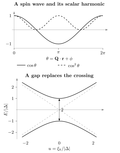
Top: a collinear spin modulation $M\cos\theta$ has a squared amplitude proportional to $\cos^2\theta$, so a scalar modulation at twice the wavevector is allowed. The scalar response need not have unit amplitude or follow this simple shape in a material. Bottom: the exactly nested two-level model has $E_\pm/|\Delta|=\pm\sqrt{u^2+1}$, where $u=\xi_k/|\Delta|$. Mixing replaces the dashed crossing by a gap $2|\Delta|$.

Commensurate and Incommensurate Order

The wave is commensurate when an integer $m$ exists such that

$$m\mathbf Q=\mathbf G$$

for a reciprocal-lattice vector $\mathbf G$. Then the phase can be locked by an invariant such as

$$F_{\mathrm{lock}} = -g_m \left( \rho_{\mathbf Q}^{\,m} +\rho_{\mathbf Q}^{*m} \right) = -2g_m\lvert\rho_{\mathbf Q}\rvert^m\cos(m\phi).$$

The continuous sliding phase is reduced to $m$ translation-related choices. An incommensurate wave has no finite $m$ and, in an ideal clean analytic description, admits a sliding phase without a finite-order lattice-locking term. Disorder and boundaries can pin it. Long-range Coulomb forces alter the phase dynamics, but should not be identified with a static pinning potential. A discrete lattice can favor nearby commensurate states. Temperature, pressure, or doping can produce lock-in transitions and discommensurations rather than a smooth change of period.

Nesting

Two Fermi-surface patches are nested by $\mathbf Q$ when translating one by $\mathbf Q$ makes it approximately parallel and coincident with another over an extended region. This enhances the phase space for low-energy particle–hole excitations.

Use the physical response to $\delta H=-fO$, with retarded susceptibility $\chi^R_{OO}(t)=+(i/\hbar)\theta(t)\langle[O(t),O(0)]\rangle$ for a Hermitian channel and Fourier factor $e^{+i\omega t}$. Here $\omega$ is angular frequency. For Bloch bands $n,m$, the corresponding bare susceptibility has the form

$$\chi_0(\mathbf q,\omega) ={} \frac{1}{N} \sum_{\mathbf k,n,m} \frac{ f(\epsilon_{m,\mathbf k+\mathbf q}) - f(\epsilon_{n\mathbf k}) }{ \hbar\omega+i0^+ +\epsilon_{n\mathbf k} -\epsilon_{m,\mathbf k+\mathbf q} } \times \left| \mathcal M_{nm}(\mathbf k,\mathbf q) \right|^2 .$$

The matrix element $\mathcal M_{nm}$ contains orbital and probe information. The low-frequency imaginary part measures near-Fermi-surface joint phase space; the static real part includes virtual transitions over a broader energy range. A geometric nesting picture can therefore disagree with the actual charge, spin, orbital, or phonon-weighted susceptibility (Johannes and Mazin, 2008).

Enhancement is not an instability

In a selected particle–hole channel $\alpha$, define $\Gamma_\alpha$ with the sign for positive feedback, so that the static response satisfies $\chi=\chi_0+\chi_0\Gamma_\alpha\chi$. With this convention, an approximate instability occurs when the largest eigenvalue of the interaction-dressed kernel reaches unity:

$$\lambda_{\max} \left[ \Gamma_{\alpha}(\mathbf q)\, \chi_0(\mathbf q,0) \right] = 1.$$

The vertex $\Gamma_\alpha$ may contain screened Coulomb, exchange, electron–phonon, orbital, and local-field effects. The matrix character matters in a multiorbital crystal. A peak in $\chi_0$ is only one factor; the interaction can favor another wavevector or channel.

For a phonon-coupled CDW, the same statement appears as a softening of a dressed phonon propagator,

$$D^{-1}(\mathbf q,\omega) = D_0^{-1}(\mathbf q,\omega) -\Pi(\mathbf q,\omega).$$

A Kohn anomaly is a nonanalyticity or pronounced softening produced by electronic response. A phonon that reaches zero frequency signals an instability of the assumed high-symmetry structure within the approximation. A broad anomaly that remains finite is evidence for coupling, not proof of static CDW order.

Why nesting is often overclaimed

Real material surfaces are rarely perfectly nested. Curvature, warping, finite lifetime, temperature, spin–orbit coupling, and orbital mismatch cut off the enhancement. In layered dichalcogenides, wavevector-dependent electron–phonon matrix elements and lattice dynamics can be as important as Fermi-surface geometry. In cuprates, charge order emerges from a correlated normal state with pseudogaps and strong momentum-dependent spectral weight, so a bare-band nesting construction is especially incomplete.

A trustworthy mechanism claim should predict the ordering wavevector, transition scale, soft mode or susceptibility evolution, orbital form factor, and response to controlled tuning. Retrofitting one observed $\mathbf Q$ to two visually parallel contours is not enough.

Peierls Instability

The Peierls problem is the controlled ideal in which nesting is strongest. Consider a one-dimensional metal with Fermi points $\pm k_{\mathrm F}$. The static susceptibility has a logarithmic singularity near $2k_{\mathrm F}$:

$$\chi_0(2k_{\mathrm F}+q,0) \sim N(0) \ln \left( \frac{\Lambda}{\lvert\hbar v_{\mathrm F}q\rvert} \right).$$

Here $q$ is a wavevector, $v_{\mathrm F}$ a physical velocity, and $\Lambda$ an energy cutoff. A lattice displacement at $Q=2k_{\mathrm F}$ creates a periodic electronic potential $\Delta_Q$. In the reduced zone, states near $k$ and $k+Q$ mix:

$$\mathcal H_k = \begin{pmatrix} \xi_k & \Delta_Q\\ \Delta_Q^{*} & \xi_{k+Q} \end{pmatrix}.$$

The reconstructed eigenvalues are

$$E_{\pm}(k) = \frac{\xi_k+\xi_{k+Q}}{2} \pm \sqrt{ \left( \frac{\xi_k-\xi_{k+Q}}{2} \right)^2 + \lvert\Delta_Q\rvert^2 }.$$

For perfect nesting, $\xi_{k+Q}=-\xi_k$ and a full gap $2\lvert\Delta_Q\rvert$ opens at the Fermi points. The electronic energy gain contains a logarithm that can overcome the elastic cost for arbitrarily weak coupling in the ideal zero-temperature mean-field limit.

Three qualifications are essential:

1. a strictly one-dimensional fluctuating system is not identical to its static mean-field solution;
2. finite-temperature order in real quasi-one-dimensional compounds requires physics beyond a strictly one-dimensional short-range model, such as interchain coupling or sufficiently long-range interactions. Discrete translation symmetry alone does not prevent thermal domain walls from destroying order in a short-range chain;
3. imperfect nesting cuts off the logarithm and restores a finite threshold.

The Peierls instability is also different from the Peierls Phase Preview, which concerns the electromagnetic gauge phase attached to a hopping amplitude.

Fermi-Surface Reconstruction

The same $2\times2$ matrix describes the simplest CDW reconstruction in any dimension, with $\Delta_Q$ replaced by a charge-order matrix element $\Phi_{\mathbf Q}(\mathbf k)$. Translation breaking folds the original Brillouin zone, hybridizes states at $\mathbf k$ and $\mathbf k+\mathbf Q$, and opens avoided crossings where their energies are close.

Imperfect nesting can leave residual Fermi pockets or other Fermi-surface sheets rather than a full gap. Photoemission may show only arcs of a pocket because coherence factors and matrix elements suppress its remaining side; an apparent arc need not be an open endpoint of a quasiparticle Fermi surface. Transport coefficients can change sign, quantum-oscillation frequencies can appear, and optical spectral weight can move from a Drude component into finite-frequency interband transitions. None of these signatures is unique to a density wave; the reconstructed states should be compared with ordering peaks and their symmetry.

For an SDW, the reconstruction matrix also acts in spin space. A collinear state can mix opposite or equal spin labels depending on the quantization convention, while a spiral mixes spin and momentum simultaneously. Spin–orbit coupling can pin the polarization and gap otherwise soft spin rotations. Itinerant Magnetism develops that matrix susceptibility and magnetic continuum in detail.

Different Routes to the Same Broken Symmetry

The same spatial pattern can arise from different interactions. An electron–phonon instability couples electronic response to a lattice distortion; intersite repulsion can favor real-space charge disproportionation; exchange can enhance a spin channel; and strongly correlated doped antiferromagnets can develop stripes. These effects can cooperate. To distinguish them, compare the soft modes, orbital content and changes under pressure or doping, rather than relying on the ordered pattern alone.

Collective Modes

Write a single complex density-wave field as

$$\Psi(\mathbf r,t) = \left[ \Psi_0+h(\mathbf r,t) \right] e^{i[\phi_0+\varphi(\mathbf r,t)]}.$$

The radial fluctuation $h$ is an amplitude mode or amplitudon. The angular fluctuation $\varphi$ is a phase mode or phason. In an ideal incommensurate neutral theory, a uniform phase shift translates the wave and costs no energy, so the phason is gapless. Commensurability and disorder add a restoring force and pin it.

Charge order couples the phason to electric fields, normal carriers, and long-range Coulomb forces. Screening, dimensionality, and pinning determine whether the mode remains low, becomes plasmon-like, or appears as a broad relaxational response. Above the transition, a soft phonon, central peak, or overdamped order-parameter fluctuation may replace a sharp collective pole.

An SDW has additional orientation modes. If spin rotation is broken continuously, transverse spin waves appear; spin–orbit anisotropy gaps or splits them. Longitudinal amplitude fluctuations usually overlap a particle–hole continuum and can be strongly damped. A sharp Raman line or pump–probe oscillation should therefore be assigned only after symmetry, polarization, temperature, and continuum coupling are checked.

Sliding transport

An incommensurate CDW can depin above a threshold electric field and contribute nonlinear collective current. Narrow-band noise, mode locking under combined dc and ac drive, and hysteretic threshold behavior are classic evidence. This is not ordinary zero-resistance superconductivity: pinning, dissipation through normal carriers, contacts, and phase slips remain central.

Competition and Coexistence with Superconductivity

Let $\rho$ denote a density-wave amplitude and $\Delta$ a uniform superconducting order parameter. The lowest local coupling consistent with both symmetries is

$$F ={} a_{\rho}\lvert\rho\rvert^2 + \frac{b_{\rho}}{2}\lvert\rho\rvert^4 + a_{\Delta}\lvert\Delta\rvert^2 + \frac{b_{\Delta}}{2}\lvert\Delta\rvert^4 + \gamma \lvert\rho\rvert^2 \lvert\Delta\rvert^2 .$$

A positive $\gamma$ expresses local competition; a negative $\gamma$ favors mutual enhancement. With $b_{\rho},b_{\Delta}>0$, a locally stable interior coexistence solution requires

$$b_{\rho}b_{\Delta}-\gamma^2>0$$

and the resulting squared amplitudes must both be positive. This determinant condition is stronger than boundedness when $\gamma$ is large and positive: because the physical variables $\lvert\rho\rvert^2$ and $\lvert\Delta\rvert^2$ are nonnegative, a large positive cross-coupling can leave the free energy bounded while favoring an axis minimum with only one order. Thus competition does not imply mutual exclusion. Spatial inhomogeneity, disorder, gradients, multiple wavevectors, and magnetic field can produce coexistence in different regions even when the local coupling is repulsive.

Microscopically, the two orders often compete for the same low-energy states. A density-wave gap reduces the density of states available for pairing; superconductivity can in turn weaken the diffraction peak below $T_c$. Conversely, a soft density-wave mode can enhance an effective pairing interaction, and partial reconstruction can leave pockets that still pair.

In underdoped YBa$_2$Cu$_3$O$_{6+x}$, x-ray measurements by Chang and collaborators (2012) show charge order that is weakened below $T_c$ and strengthened when magnetic field suppresses superconductivity. This is direct evidence for competition in that material and regime, not a universal sign of $\gamma$ for every density wave. Stripe-ordered La-based cuprates demonstrate that spin order, charge order, lattice symmetry, and superconducting coherence can be intertwined in still more structured ways.

A pair-density wave is a spatial modulation of the pair field, not merely a CDW coexisting with uniform superconductivity. Couplings can induce secondary charge harmonics, but the pair order requires a pair-sensitive diagnostic.

How Measurements Reveal the Wave

Probe	What it reveals and what needs care
X-ray diffraction	Satellites and correlation lengths; nonresonant intensity may mainly reflect atomic displacement. Resonant energy and polarization dependence help resolve orbital content.
Neutron diffraction	Magnetic satellites and spin orientation; distinguish nuclear scattering and slowly fluctuating moments.
Photoemission	Folded bands and avoided crossings; include surfaces, domains and matrix elements.
Scanning tunneling microscopy	Spatial phase and defects; separate density-wave order from dispersing quasiparticle interference and surface effects.
Optical and transport probes	Reconstructed carriers, pinning and nonlinear sliding; an anomaly alone does not identify the broken symmetry.
Local magnetic or nuclear probes	Internal fields, charge environments and fluctuation times; disorder can also broaden lines.

A peak has both a spatial width and an energy width. A finite-width momentum peak indicates a finite correlation length after instrumental broadening is removed. A signal called elastic is static only within the instrument’s time resolution. Comparing several time windows can distinguish stable order from slow fluctuations. True long-range order requires an appropriate correlation or finite-size limit, as illustrated in exercise 6; a large raw peak is insufficient.

Material Examples

Quasi-one-dimensional conductors

Compounds such as blue bronze and NbSe$_3$ display multiple classic CDW signatures: superlattice peaks, partial electronic gaps, pinned collective response, threshold conduction, and narrow-band noise. Their anisotropy makes the Peierls language useful, while interchain coupling and disorder explain why the real transition is not a strictly one-dimensional mean-field theorem.

Layered transition-metal dichalcogenides

Materials such as 2H-NbSe$_2$ combine charge order, soft phonons, multiband electronic structure, and superconductivity. The ordering wavevector is not explained reliably by Fermi-surface geometry alone; momentum-dependent electron–phonon coupling and lattice dynamics are part of the explanation. Weber and collaborators (2011) observed softening over an extended momentum region, an instructive contrast with an ideal sharp nesting anomaly.

Chromium

Chromium is the canonical itinerant SDW metal. Incommensurate magnetic order, a concomitant charge and strain modulation, reconstructed electronic structure, and pressure or alloy dependence can be related to electron and hole Fermi-surface sheets. Even here, quantitative theory requires more than a nesting cartoon.

Cuprates

Cuprate charge order and spin stripes live in a strongly correlated, often pseudogapped background. Their wavevectors, orbital form factors, short correlation lengths, field response, and relation to superconductivity vary across families. The t–J Model supplies one projected strong-coupling language, but the observed density wave is not thereby reduced to weak-coupling nesting or to one universal stripe mechanism.

Exercises

1. Translation and time reversal

For a scalar CDW amplitude $\rho_{\mathbf Q}$ and a collinear SDW amplitude $\mathbf M_{\mathbf Q}$, determine their transformation under translation by $\mathbf a$ and time reversal. Which symmetries are necessarily broken by a generic incommensurate state?

Solution

Translation gives the phase factors

$$\rho_{\mathbf Q} \mapsto e^{i\mathbf Q\cdot\mathbf a}\rho_{\mathbf Q}, \qquad \mathbf M_{\mathbf Q} \mapsto e^{i\mathbf Q\cdot\mathbf a}\mathbf M_{\mathbf Q}.$$

Time reversal acts on the physical profiles without reflecting space:

$$\rho_{\mathbf Q}\mapsto\rho_{\mathbf Q}, \qquad \mathbf M_{\mathbf Q}\mapsto-\mathbf M_{\mathbf Q}.$$

The operator identities $\mathcal T\widehat\rho_{\mathbf Q}\mathcal T^{-1}=\widehat\rho_{-\mathbf Q}$ and $\mathcal T\widehat{\mathbf S}_{\mathbf Q}\mathcal T^{-1}=-\widehat{\mathbf S}_{-\mathbf Q}$ contain a conjugated wavevector because $\mathcal T$ is antiunitary. The transformed expectation value is conjugated once more. The reality relation $\rho_{-\mathbf Q}=\rho_{\mathbf Q}^{*}$ should therefore not be mistaken for a time-reversal shift of the physical charge pattern.

A generic incommensurate CDW breaks lattice translation but need not break time reversal. A collinear SDW breaks translation and time reversal; without spin–orbit pinning it also breaks continuous spin rotation down to rotations about the ordered axis. Point-group symmetry may also break if one member of a symmetry-related star of wavevectors is selected.

2. Density-wave reconstruction

Diagonalize

$$\mathcal H_k = \begin{pmatrix} \xi_k & \Delta\\ \Delta^{*} & \xi_{k+Q} \end{pmatrix}$$

and show that perfect nesting produces a gap $2\lvert\Delta\rvert$.

Solution

The characteristic equation gives

$$E_{\pm} = \frac{\xi_k+\xi_{k+Q}}{2} \pm \sqrt{ \left( \frac{\xi_k-\xi_{k+Q}}{2} \right)^2 + \lvert\Delta\rvert^2 }.$$

Under perfect nesting, $\xi_{k+Q}=-\xi_k$, so

$$E_{\pm} = \pm\sqrt{\xi_k^2+\lvert\Delta\rvert^2}.$$

At the original Fermi crossing $\xi_k=0$, the upper and lower branches lie at $\pm\lvert\Delta\rvert$. Their separation is therefore $2\lvert\Delta\rvert$.

3. Cutoff of the Peierls singularity

The ideal one-dimensional susceptibility contains

$$\chi_0(2k_{\mathrm F}+q,0) \sim N(0)\ln \left( \frac{\Lambda}{\lvert\hbar v_{\mathrm F}q\rvert} \right).$$

Give three physical effects that replace the vanishing denominator by a finite scale, and state their consequence for the instability.

Solution

Finite temperature smears the Fermi edge and supplies a scale of order $k_{\mathrm B}T$. A finite quasiparticle scattering rate supplies $\hbar/\tau$. Transverse hopping or Fermi-surface curvature produces an imperfect-nesting mismatch $\delta_{\mathrm{nest}}$. Schematically,

$$\lvert\hbar v_{\mathrm F}q\rvert \longrightarrow \max \left( \lvert\hbar v_{\mathrm F}q\rvert, k_{\mathrm B}T, \frac{\hbar}{\tau}, \delta_{\mathrm{nest}} \right).$$

At a fixed nonzero cutoff, the logarithm remains finite and the interaction must exceed a corresponding threshold in this mean-field criterion. Temperature is a tunable cutoff: if it is the only cutoff, reducing it can recover an exponentially small transition scale for arbitrarily weak coupling within mean field. A nonzero nesting mismatch that remains at zero temperature is different. Neither statement eliminates one-dimensional fluctuations.

4. Charge harmonic induced by a collinear SDW

Let $\mathbf S(\mathbf r)=\mathbf M_0\cos(\mathbf Q\cdot\mathbf r+\phi)$. Show that the scalar $\mathbf S^2$ contains a component at $2\mathbf Q$, and explain why the same conclusion can fail for a circular spiral.

Solution

Using $\cos^2\theta=(1+\cos2\theta)/2$,

$$\mathbf S^2(\mathbf r) = \frac{\lvert\mathbf M_0\rvert^2}{2} \left[ 1+ \cos(2\mathbf Q\cdot\mathbf r+2\phi) \right].$$

A scalar charge or lattice field can therefore couple linearly to the $2\mathbf Q$ harmonic.

For a circular spiral, write

$$\mathbf M_{\mathbf Q} = M \left( \widehat{\mathbf x} -i\widehat{\mathbf y} \right).$$

With the real-part convention used above, this gives $\mathbf S(\mathbf r)=M[\widehat{\mathbf x}\cos(\mathbf Q\cdot\mathbf r)+\widehat{\mathbf y}\sin(\mathbf Q\cdot\mathbf r)]$. Then $\mathbf M_{\mathbf Q}\cdot\mathbf M_{\mathbf Q}=0$. The spin magnitude is spatially constant, so the simplest quadratic mechanism does not induce a $2\mathbf Q$ charge modulation.

5. Homogeneous coexistence with superconductivity

For the Landau free energy above, set $x=\lvert\rho\rvert^2$ and $y=\lvert\Delta\rvert^2$. Solve for a stationary coexistence state and state the stability and positivity conditions.

Solution

The stationarity equations are

$$\begin{pmatrix} b_{\rho} & \gamma\\ \gamma & b_{\Delta} \end{pmatrix} \begin{pmatrix} x\\y \end{pmatrix} = - \begin{pmatrix} a_{\rho}\\a_{\Delta} \end{pmatrix}.$$

Inverting gives

$$\begin{aligned} x &= \frac{ -a_{\rho}b_{\Delta} +\gamma a_{\Delta} }{ b_{\rho}b_{\Delta}-\gamma^2 }, \\ y &= \frac{ -a_{\Delta}b_{\rho} +\gamma a_{\rho} }{ b_{\rho}b_{\Delta}-\gamma^2 }. \end{aligned}$$

The Hessian in the interior variables $(x,y)$ is positive definite when $b_{\rho}>0$, $b_{\Delta}>0$, and $b_{\rho}b_{\Delta}>\gamma^2$. Homogeneous coexistence additionally requires $x>0$ and $y>0$. A positive $\gamma$ suppresses both amplitudes relative to uncoupled values but does not automatically make either vanish. If $\gamma>\sqrt{b_{\rho}b_{\Delta}}$, the quartic energy is still bounded on the physical quadrant $x,y\geq0$, but the interior stationary point is not a coexistence minimum.

6. Peak growth versus long-range order

For $N=L^d$ sites, define

$$S(\mathbf Q) = \frac{1}{N} \sum_{i,j} e^{i\mathbf Q\cdot(\mathbf r_i-\mathbf r_j)} \langle O_i O_j\rangle.$$

How does $S(\mathbf Q)$ scale for true long-range order, finite-correlation-length order, and algebraic correlations $\langle O(\mathbf r)O(0)\rangle\sim r^{-\eta}$?

Solution

Let $m_{\mathbf Q}^2$ denote the long-range Fourier component of the correlation at the chosen peak, including the normalization appropriate to the real-space modulation. Its coherent contribution to the double sum is $N^2m_{\mathbf Q}^2$, so

$$S(\mathbf Q)\sim Nm_{\mathbf Q}^2.$$

Thus $S(\mathbf Q)/N\to m_{\mathbf Q}^2$. For a simple incommensurate cosine of amplitude $A$, averaging its global phase gives $m_{\mathbf Q}^2=A^2/4$ at either satellite.

For finite correlation length $\xi$, each site correlates coherently with only a volume of order $\xi^d$, so $S(\mathbf Q)$ approaches a size-independent value proportional to $\xi^d$ once $L\gg\xi$.

For algebraic correlations, integrate $r^{-\eta}$ over a volume of radius $L$:

$$S(\mathbf Q) \sim L^{d-\eta}$$

for $0<\eta<d$. The peak diverges but remains subextensive, so $S(\mathbf Q)/N\sim L^{-\eta}\to0$. A growing raw peak is therefore not sufficient evidence for long-range order.

Related Topics

• Itinerant Magnetism develops the matrix susceptibility and the SDW example of chromium.
• Competing Orders studies the phase diagrams of coupled order parameters.
• Pair-Density Waves and Exotic Orders distinguishes finite-momentum pair order from charge order.
• Transition-Metal Dichalcogenides covers semiconducting monolayers and moiré systems, distinct from the metallic examples here.

References

• J. Chang, E. Blackburn, A. T. Holmes, et al., “Direct observation of competition between superconductivity and charge density wave order in YBa$_2$Cu$_3$O$_{6.67}$,” Nature Physics 8, 871–876 (2012).
• R. Comin and A. Damascelli, “Resonant x-ray scattering studies of charge order in cuprates,” Annual Review of Condensed Matter Physics 7, 369–405 (2016).
• E. Fawcett, “Spin-density-wave antiferromagnetism in chromium,” Reviews of Modern Physics 60, 209–283 (1988).
• E. Fradkin, S. A. Kivelson, and J. M. Tranquada, “Colloquium: Theory of intertwined orders in high temperature superconductors,” Reviews of Modern Physics 87, 457–482 (2015).
• G. Grüner, “The dynamics of charge-density waves,” Reviews of Modern Physics 60, 1129–1181 (1988).
• M. D. Johannes and I. I. Mazin, “Fermi surface nesting and the origin of charge density waves in metals,” Physical Review B 77, 165135 (2008).
• M. D. Johannes, I. I. Mazin, and C. A. Howells, “Fermi-surface nesting and the origin of the charge-density wave in NbSe$_2$,” Physical Review B 73, 205102 (2006).
• W. Kohn, “Image of the Fermi surface in the vibration spectrum of a metal,” Physical Review Letters 2, 393–394 (1959).
• P. A. Lee, T. M. Rice, and P. W. Anderson, “Fluctuation effects at a Peierls transition,” Solid State Communications 14, 703–709 (1974).
• P. B. Littlewood and C. M. Varma, “Amplitude collective modes in superconductors and their coupling to charge-density waves,” Physical Review B 26, 4883–4893 (1982).
• P. Monceau, “Electronic crystals: An experimental overview,” Advances in Physics 61, 325–581 (2012).
• A. W. Overhauser, “Spin density waves in an electron gas,” Physical Review 128, 1437–1452 (1962).
• J. M. Tranquada, B. J. Sternlieb, J. D. Axe, Y. Nakamura, and S. Uchida, “Evidence for stripe correlations of spins and holes in copper oxide superconductors,” Nature 375, 561–563 (1995).
• F. Weber, S. Rosenkranz, J.-P. Castellan, et al., “Extended phonon collapse and the origin of the charge-density wave in 2H-NbSe$_2$,” Physical Review Letters 107, 107403 (2011).
• J. A. Wilson, F. J. Di Salvo, and S. Mahajan, “Charge-density waves and superlattices in the metallic layered transition metal dichalcogenides,” Advances in Physics 24, 117–201 (1975).