Neutron Scattering

Neutron scattering measures how a sample changes a neutron’s direction, energy, and sometimes spin. Ångström wavelengths resolve atomic arrangements; millielectronvolt energy changes reveal phonons, magnetic excitations, and slow motion. Nuclear scattering probes atomic positions, while magnetic scattering probes the component of electronic magnetization perpendicular to the transferred wavevector.

This guide develops slow-neutron measurements of bulk condensed matter, from the scattering triangle to spectra and their interpretation. The central task is to predict counts from a correlation function, including the coupling, geometry, and instrument resolution. A missing branch may be invisible in the chosen geometry, and a broad peak may be broadened by the instrument. Neither feature can be interpreted from its shape alone.

Required background. Reciprocal Lattice supplies momentum-transfer coordinates and reciprocal-lattice indexing. Structure Factors supplies the static and dynamic correlation functions underlying elastic and inelastic intensity. How Quantum Matter Is Measured supplies detector normalization, resolution and competing-model checks.

Neutron cross sections and material correlations

A neutron event determines an outgoing direction and, in a spectrometer, an outgoing energy. Many events build a cross section: the probability of scattering into a specified solid angle and energy interval, expressed as an effective area. Interference between scattering from different sites makes this cross section sensitive to spatial correlations. Exchanging energy with the sample makes it sensitive to their time dependence.

The correlation functions are developed in Structure Factors. Here we connect them to measurable intensities. The treatment starts with single scattering in the Born approximation; absorption, repeated scattering, and strong-reflection extinction require additional corrections. Squires (2012) and Berk (1993) develop this framework in detail.

Why neutrons probe nuclei and spins

Matching material length and energy scales

For a free neutron of mass $m_n$,

$$k = \frac{2\pi}{\lambda}, \qquad E = \frac{\hbar^2k^2}{2m_n}.$$

Useful numerical forms are

$$\begin{aligned} E[\mathrm{meV}] &\simeq 2.072\, \bigl( k[\mathrm{\mathring A}^{-1}] \bigr)^2, \\ E[\mathrm{meV}] &\simeq \frac{81.81}{ \bigl( \lambda[\mathrm{\mathring A}] \bigr)^2 }. \end{aligned}$$

Cold and thermal neutrons therefore place lattice spacings, phonons, spin waves, crystal-field transitions, diffusion, and slow collective motion within one kinematic range. Hot neutrons extend the accessible energy and momentum transfers; cold neutrons improve access to long wavelengths and low energies. Flux and resolution change with that choice.

Neutrons are electrically neutral, so they can penetrate sample environments and bulk crystals more deeply than charged-particle probes. Penetration is material and wavelength dependent, however. Absorbing isotopes, thick samples, cryostat walls, pressure cells, and strong incoherent scatterers can dominate the usable transmission.

Short-range nuclear coupling

At slow-neutron energies, nuclear scattering is represented by an effective Fermi pseudopotential,

$$V_N(\mathbf r) = \frac{2\pi\hbar^2}{m_n} \sum_j \widehat b_j\, \delta \left( \mathbf r-\mathbf R_j \right),$$

Here $\widehat b_j$ is a bound scattering-length operator acting on the neutron and nuclear spins. For a specified total-spin scattering channel it reduces to a channel scattering length; averaging the amplitude over an unpolarized isotope/spin mixture gives the coherent length. Unlike an x-ray form factor, the scattering length does not grow monotonically with atomic number. Neighboring elements or isotopes can have very different amplitudes and signs. This gives neutrons unusual sensitivity to light atoms and enables isotope contrast.

For an unpolarized statistical mixture, define averages over the isotope distribution and the initial spin density matrix, with final spins summed:

$$\overline b = \left\langle \widehat b\right\rangle, \qquad \overline{\lvert b\rvert^2} = \left\langle\widehat b^\dagger\widehat b\right\rangle.$$

The idealized bound cross sections separate as

$$\begin{aligned} \sigma_{\mathrm{coh}} &= 4\pi \left| \overline b \right|^2, \\ \sigma_{\mathrm{inc}} &= 4\pi \left( \overline{\lvert b\rvert^2} - \left| \overline b \right|^2 \right). \end{aligned}$$

For independently distributed isotope and nuclear-spin states, uncorrelated with atomic motion, coherent scattering retains interference between different nuclei; the incoherent term is proportional to self correlations. Correlated isotope occupations or nuclear-spin order require their own distinct-site correlations and cannot be reduced to this simple separation. It can be the desired signal in diffusion or vibrational-density measurements, but it is a background for many diffraction and collective-mode experiments.

NIST scattering tables illustrate the practical stakes: hydrogen’s thermal incoherent cross section is about $80.3$ barns, whereas deuterium’s is about $2.05$ barns. Deuteration can reduce incoherent background by nearly a factor of forty, but it also changes mass, zero-point motion, exchange pathways, and sometimes the phase itself. An isotopic substitution is part of the sample definition, not a free background correction.

Magnetic dipole coupling

The neutron magnetic moment couples to the magnetic field generated by electronic spin and orbital magnetization. In reciprocal space, dipolar geometry makes the neutron sensitive only to magnetization perpendicular to $\mathbf Q$. For one type of magnetic ion with an isotropic scalar $g$ factor and a factorizable magnetic form factor, unpolarized inelastic scattering has the tensor dependence

$$\frac{d^2\sigma_{\mathrm{mag}}}{ d\Omega\,dE_f } \propto \frac{k_f}{k_i} \times \left| f(\mathbf Q) \right|^2 \times \sum_{\alpha,\beta} \left( \delta_{\alpha\beta} - \widehat Q_\alpha \widehat Q_\beta \right) \times S^{\alpha\beta} \left( \mathbf Q,\omega \right).$$

Here $S^{\alpha\beta}$ is the correlation tensor of dimensionless spins; the proportionality suppresses the magnetic coupling constant, $g^2$, the number of spins, and the energy-normalization factor described below. The normalized form factor $f(\mathbf Q)$ describes the spatial extent of the ion’s magnetization and usually decreases with $\lvert\mathbf Q\rvert$. With an anisotropic $g$ tensor, form and project correlations of the moment $\boldsymbol\mu=-\mu_{\mathrm B}g\mathbf S$, including the two corresponding $g$ factors. Several inequivalent ions also require their separate form factors and basis interference; a single scalar $f$ need not suffice. The transverse projector can extinguish a fluctuation parallel to $\mathbf Q$. Neither suppression means that the underlying mode is absent.

Nuclear and magnetic amplitudes can coexist at the same reciprocal-space point. Incident polarization and analysis of the outgoing neutron spin can separate spin-flip and non-spin-flip channels, identify chiral or antisymmetric correlations, and expose nuclear–magnetic interference. The separation depends on the chosen polarization axes, flipping ratio, guide fields, domains, and depolarization corrections. Spin-flip does not mean exclusively electronic magnetism: for randomly oriented, unpolarized nuclear spins, two thirds of the nuclear spin-incoherent intensity is spin-flip and one third is non-spin-flip. Isotope incoherence alone is non-spin-flip. These fractions assume ideal polarization analysis; magnetic intensity can enter either channel depending on its direction (Moon, Riste, and Koehler, 1969).

From detector events to a scattering triangle

A time-of-flight instrument records detector position and arrival time relative to the incident pulse. Flight paths and the selected incident-energy band convert those events into outgoing wavevectors. A crystal analyzer instead selects a final wavelength before the neutron reaches the detector. In either case, calibration fixes the coordinates; monitor counts, detector efficiency, and sample transmission fix the intensity scale.

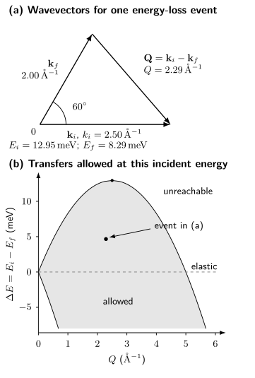
The same event appears in both panels: $k_i=2.50\,\mathrm{\mathring A}^{-1}$, $k_f=2.00\,\mathrm{\mathring A}^{-1}$, and $\phi=60^\circ$ give $Q=2.29\,\mathrm{\mathring A}^{-1}$ and energy loss $\Delta E=4.66\,\mathrm{meV}$. The shaded region allows all scattering angles at fixed $E_i=12.95\,\mathrm{meV}$; actual detector coverage and crystal orientation restrict it further. Positive transfer creates excitations in the sample. Negative transfer draws energy from the sample. An unshaded region cannot be reached at this incident energy, even if the material has an excitation there.

Scattering Kinematics

The transferred wavevector and energy, with positive signs into the sample, are

$$\mathbf Q = \mathbf k_i-\mathbf k_f, \qquad \hbar\omega = E_i-E_f.$$

The physical momentum transfer is $\hbar\mathbf Q$, not $\mathbf Q$ itself. Positive $\omega$ means the neutron lost energy and created or excited something in the sample. Negative $\omega$ means the neutron gained energy by annihilating a thermally occupied excitation. Some diffraction and crystallography software uses the opposite sign for $\mathbf Q$; the intensity may look unchanged while complex structure factors and polarization conventions do not.

If $\phi$ is the angle between the incident and final wavevectors,

$$Q^2 = k_i^2+k_f^2 - 2k_i k_f\cos\phi.$$

For elastic scattering, $k_i=k_f=k$ and

$$Q = 2k \sin \left( \frac{\phi}{2} \right).$$

In a crystal, it is useful to decompose

$$\mathbf Q = \boldsymbol\tau+\mathbf q,$$

where $\boldsymbol\tau$ is a reciprocal-lattice vector and $\mathbf q$ lies in a chosen Brillouin zone. A magnetic structure can have a larger real-space unit cell and a different reciprocal vector $\boldsymbol\tau_m$. The instrument measures absolute $\mathbf Q$; reducing it into a chemical or magnetic zone is an analysis convention that must be stated.

At fixed $E_i$, write $\Delta E=\hbar\omega$ and require

$$\begin{aligned} E_f&=E_i-\Delta E\geq0,\\ |k_i-k_f|&\leq Q\leq k_i+k_f. \end{aligned}$$

These triangle inequalities give the shaded region in the figure. Energy and momentum transfer are coupled by the neutron dispersion. At fixed $E_i$, not every desired $(\mathbf Q,\omega)$ point is reachable at every detector angle. Sample rotation, incident energy, analyzer setting, and scattering plane determine coverage. A visually empty region can be kinematically inaccessible rather than physically dark.

Elastic, Quasielastic, and Inelastic Scattering

Elastic diffraction

Elastic scattering has $\omega=0$ within resolution. Long-range periodic nuclear order produces Bragg peaks at reciprocal vectors. A nuclear unit-cell amplitude is

$$F_N(\mathbf Q) = \sum_d o_d b_d e^{-W_d(\mathbf Q)} e^{i\mathbf Q\cdot\mathbf r_d},$$

where $o_d$ is occupancy and $e^{-W_d}$ is the Debye–Waller amplitude. After Lorentz, multiplicity, absorption, extinction, preferred-orientation, and instrument corrections, integrated Bragg intensity constrains $\lvert F_N\rvert^2$.

Magnetic order similarly gives elastic peaks through a magnetic structure factor projected perpendicular to $\mathbf Q$. Magnetic peaks can occur at nuclear-forbidden positions or coincide with nuclear reflections. Their temperature dependence and decay with magnetic form factor help, but polarized analysis or a full magnetic refinement may be needed.

A Bragg peak establishes a nonzero spatial Fourier component averaged over the probe’s time window. It does not by itself identify the microscopic interaction that selected the order. Peak width constrains correlation length only after deconvolving instrument resolution, mosaic, strain, finite domain size, and sample-shape effects.

Quasielastic scattering

Slow fluctuations appear as intensity centered near $\omega=0$ with finite width. Diffusion, domain motion, spin relaxation, glassy dynamics, and rotational or translational molecular motion can all be quasielastic. If the intrinsic width is narrower than the instrument resolution, the signal is experimentally elastic even if the microscopic process is dynamic.

For example, a normalized classical correlation $F(t)=e^{-|t|/\tau}$ has

$$S(\omega)=\frac{1}{2\pi}\int dt\,e^{i\omega t}F(t) =\frac{\tau}{\pi(1+\omega^2\tau^2)}.$$

Its energy half width is $\Gamma_E=\hbar/\tau$. This symmetric Lorentzian is a classical low-energy approximation, $|\hbar\omega|\ll k_{\mathrm B}T$; at larger transfer a quantum spectrum must satisfy detailed balance, below. A narrower peak corresponds to slower relaxation, but only after instrumental broadening has been separated.

Backscattering and neutron spin echo access much slower timescales than conventional thermal-neutron spectroscopy. Comparing instruments therefore requires a time-window statement. “Static” means static on the stated resolution scale.

Inelastic scattering

Inelastic events have resolvable $\omega\ne0$. They can reveal:

• phonons and molecular vibrations through nuclear displacement correlations;
• magnons, paramagnons, and crystal-field transitions through magnetic correlations;
• diffusion and relaxational continua;
• multiphonon and multimagnon states;
• fractionalized or emergent-gauge continua;
• hybrid magnetoelastic modes containing both nuclear and magnetic weight.

Mode energy, intrinsic linewidth, and integrated spectral weight are distinct observables. A constant-$\mathbf Q$ scan, a constant-energy slice, and a cut following a dispersion convolve the four-dimensional resolution differently.

Dynamic Structure Factors and the Measured Cross Section

For Hermitian local observables $O_j$ at positions $\mathbf R_j$, define $O_{\mathbf Q}=\sum_j e^{-i\mathbf Q\cdot\mathbf R_j}O_j$, so $O_{\mathbf Q}^\dagger=O_{-\mathbf Q}$. A per-particle convention, with $\omega$ an angular frequency and $N$ the number of sites, is

$$S_{OO}(\mathbf Q,\omega) = \frac{1}{2\pi N} \int_{-\infty}^{\infty} dt\, \times e^{i\omega t} \left\langle O_{\mathbf Q}(t) O_{-\mathbf Q}(0) \right\rangle.$$

Density, isotope-weighted displacement, and magnetization define different structure factors. For a spectrum per unit energy, use

$$\begin{aligned} S_E(\mathbf Q,\Delta E)&=\frac{1}{\hbar} S_{OO}(\mathbf Q,\Delta E/\hbar),\\ S_E\,d(\Delta E)&=S_{OO}\,d\omega. \end{aligned}$$

This factor matters when converting a cross section per meV to a sum rule. State also whether the normalization is per formula unit or magnetic ion and which spin components are included. Structure Factors explains connected correlations, elastic delta functions, and response functions.

For the Hermitian channel just defined, thermal equilibrium implies

$$S(\mathbf Q,-\omega) = e^{-\beta\hbar\omega} S(-\mathbf Q,\omega).$$

The relation compares opposite momenta as well as opposite energies. A comparison at the same $\mathbf Q$ additionally needs $S(-\mathbf Q,\omega)=S(\mathbf Q,\omega)$, for example from the relevant inversion symmetry. The Boltzmann ratio applies to the structure factor after removing the $k_f/k_i$ and other measurement factors. This makes detailed balance a useful diagnostic. Failure can signal an incorrect sign convention, temperature mismatch, background subtraction error, detector normalization problem, or genuine nonequilibrium.

For a fixed incident state and sample orientation, a single-scattering model for the expected counts in detector bin $x$ is

$$C_x=T_{\mathrm{run}}\Phi \int d\Omega\,dE_f\, \times\epsilon\,\mathcal A\,R_x(\Omega,E_f) \frac{d^2\sigma}{d\Omega\,dE_f} +B_x.$$

Here $\Phi$ is incident flux per area per time, the cross section is for the illuminated sample, $\epsilon$ is detector efficiency, and $\mathcal A$ describes attenuation in a sample-geometry approximation. The dimensionless $R_x$ is the probability that an outgoing neutron with these coordinates is assigned to bin $x$, including resolution and acceptance; $B_x$ is the expected background count. Thus flux times time times cross-sectional area gives a count. A real incident bandwidth and divergence require an additional average over incident states. A calculation using a per-ion cross section also needs the number of illuminated ions.

The integration measure must match the differential cross section. Resampling into $(\mathbf Q,\omega)$ coordinates requires the corresponding Jacobian and accessible-manifold or orientation treatment; replacing $d\Omega\,dE_f$ by $d^3Q\,d\omega$ without those factors is incorrect. The resolution distribution can be tilted in momentum–energy space, so a steep sharp branch can appear broad. We calculate that effect in Exercise 5.

Instrument Architectures

Diffraction

A diffractometer emphasizes elastic intensity. Powder diffraction trades directional information for orientational averaging and broad reciprocal-space coverage. Single-crystal diffraction retains directions and domain information but requires an orientation model and adequate reciprocal-space sampling. Energy-integrating detectors can admit inelastic contamination; filters and wavelength discrimination matter.

Triple-axis spectroscopy

A triple-axis spectrometer uses:

1. a monochromator to select $\mathbf k_i$;
2. sample rotation and scattering angle to choose $\mathbf Q$;
3. an analyzer to select $\mathbf k_f$ before detection.

Holding $E_f$ fixed is common because it stabilizes analyzer and detector conditions, but fixed-$E_i$ operation is also possible. Triple-axis instruments make targeted trajectories through $(\mathbf Q,\omega)$ with tunable collimation and focusing. They are efficient when the expected signal is localized, and inefficient for discovering an unknown response over a large volume.

Higher-order wavelength contamination, monitor sensitivity, analyzer harmonics, focusing, and resolution geometry must be included. A scan coordinate is not necessarily orthogonal to a dispersing branch.

Time-of-flight spectroscopy

At a pulsed source, choppers select an incident-energy band and detector arrival times infer $E_f$. A direct-geometry instrument usually fixes $E_i$ and records broad angular and energy coverage simultaneously. Rotating a single crystal builds a four-dimensional dataset. Indirect-geometry instruments instead constrain $E_f$ with analyzer crystals.

Time-of-flight coverage is broad but highly nonuniform. Detector gaps, frame overlap, chopper transmission, incident flux, and the $k_f/k_i$ phase-space factor shape the raw map. Merging several $E_i$ settings can extend dynamic range only if their normalizations and resolutions are retained.

High-resolution and polarized methods

• Backscattering uses near-$180^\circ$ Bragg geometry for very fine energy resolution over a restricted range.
• Neutron spin echo encodes energy transfer in a Larmor phase and measures an intermediate scattering function over long times.
• Polarization analysis resolves spin-flip and non-spin-flip channels, magnetic components, and nuclear–magnetic interference.
• Small-angle scattering targets structures much larger than an atomic spacing near $Q=0$.
• Reflectometry resolves depth profiles normal to an interface under a layered optical model.

Instrument names are not interchangeable labels for $S(\mathbf Q,\omega)$. Each architecture samples and convolves a different region.

Phonons

For one-phonon coherent nuclear scattering at

$$\mathbf Q = \boldsymbol\tau+\mathbf q,$$

choose polarization vectors normalized by $\sum_d\mathbf e_{d\nu}^*\cdot\mathbf e_{d\nu}=1$ and the creation matrix element

$$\langle\nu,\mathbf q|\mathbf u_{ld}|0\rangle =\sqrt{\frac{\hbar}{2N_cM_d\omega_\nu}} \mathbf e_{d\nu}^*(\mathbf q)e^{-i\mathbf q\cdot\mathbf R_l}.$$

$l$ labels the $N_c$ unit cells, $d$ a basis atom of mass $M_d$, and $\mathbf u_{ld}$ its displacement. With this explicit phase convention, the mode-dependent amplitude contains

$$F_\nu(\mathbf Q) = \sum_d \frac{ b_d e^{-W_d(\mathbf Q)} }{ \sqrt{M_d} } \left[ \mathbf Q\cdot \mathbf e_{d\nu}^*(\mathbf q) \right] e^{i\mathbf Q\cdot\mathbf r_d}.$$

The corresponding creation intensity scales schematically as

$$I_\nu^{(+)} \propto \frac{k_f}{k_i} \frac{ \left| F_\nu(\mathbf Q) \right|^2 }{ \omega_\nu(\mathbf q) } \left[ n_{\mathrm B} \left( \omega_\nu \right) + 1 \right],$$

before multiphonon terms and resolution convolution.

This kernel explains why:

• a mode can disappear when $\mathbf Q\cdot\mathbf e_{d\nu}=0$;
• basis atoms interfere differently in different reciprocal zones;
• light atoms can have large displacement amplitudes;
• creation remains possible at zero temperature, while annihilation loses Bose population;
• phonon intensity often grows with $Q$ through the displacement factor even when a magnetic form factor is falling.

Measuring the same reduced $\mathbf q$ in several zones is therefore a polarization and eigenvector test, not redundant repetition. A fitted force-constant model should reproduce frequencies and absolute or consistently normalized intensities across zones. Phonons develops the dynamical matrix and explains how the eigenvectors and frequencies are calculated.

Powder incoherent measurements can approximate a neutron-weighted vibrational density of states. The weights depend roughly on scattering cross section divided by mass, and multiphonon subtraction is model dependent. Calling the result “the phonon DOS” without its neutron weighting can mislead comparisons with calculations or other probes.

Magnons and Magnetic Excitations

A magnetic mode contributes through the same transverse projector and form factor that govern the general magnetic cross section. For a branch $\nu$, the intensity contains a matrix element of the magnetization operator,

$$\mathcal M_\nu^\alpha(\mathbf Q) = \left\langle \nu,\mathbf q \middle| M_{-\mathbf Q}^\alpha \middle| 0 \right\rangle,$$

With the Fourier convention used above, the excitation is created by $M_{-\mathbf Q}^\alpha$. The amplitudes combine as

$$\sum_{\alpha,\beta} \left( \delta_{\alpha\beta} - \widehat Q_\alpha\widehat Q_\beta \right) \mathcal M_\nu^\alpha \mathcal M_\nu^{\beta *}.$$

Peak positions alone do not determine an exchange Hamiltonian. Different exchange parameters can produce similar peak positions. Intensities across zones, sublattice interference, polarization, domain populations, and field dependence often distinguish them. A useful refinement predicts these alongside the branches and their resolution-convolved widths.

Elastic magnetic diffraction should establish the reference structure before a harmonic magnon model is fitted. If the ordered state is not stationary under the proposed Hamiltonian, a numerically attractive dispersion fit is physically inconsistent. Spin Waves and Magnons develops that model-validation route.

At finite temperature or strong interaction, a magnon can shift, broaden, decay into several particles, or hybridize with a phonon. Avoided crossings accompanied by exchanged nuclear and magnetic intensity are stronger evidence for magnetoelastic hybridization than two nearby peak positions alone. Polarization analysis, reciprocal-zone dependence, field tuning, and isotope substitution can separate channels.

Absolute normalization allows a particularly useful check. For one dimensionless spin of fixed length $S$ on each of $N$ Bravais-lattice sites, use the per-spin structure factor above and sum over the $N$ wavevectors in one full Brillouin zone. Then

$$\frac{1}{N} \sum_{\mathbf q} \sum_\alpha \int_{-\infty}^{\infty} d\omega\, S^{\alpha\alpha}(\mathbf q,\omega) = S(S+1),$$

The integral includes both energy signs and any elastic weight, and the sum includes all three spin components. It is the identity $\langle\mathbf S_j^2\rangle=S(S+1)$ expressed in momentum and frequency. An isotropic physical-moment sum has an additional factor $(g\mu_{\mathrm B})^2$; anisotropic moments require their tensor instead. Neutrons measure a transverse projection, so a single geometry does not collect all three components. A truncated low-energy multiplet may also omit transitions needed for the full ionic moment; see Magnetic Moments. Exercise 6 makes the missing-component issue explicit.

Spin-Liquid Continua

A local spin operator in a fractionalized phase can create two or more spinons or Majorana-like excitations. Their allowed total energies at fixed momentum fill a continuum rather than a single branch. Inelastic neutron scattering is therefore a natural probe of fractionalization.

The converse is false. Broad magnetic intensity can also arise from:

• two-magnon and higher-particle states;
• decay of a conventional mode into an allowed continuum;
• disorder-broadened local excitations or random singlets;
• overlapping crystal-field transitions;
• unresolved dispersive branches or domains;
• phonon and multiphonon backgrounds;
• multiple scattering and sample-environment subtraction errors.

To test a fractionalized interpretation, first separate magnetic weight from nuclear background, then compare its momentum-dependent boundaries, polarization, and field evolution with competing models. Repeat at another incident energy or resolution to expose overlapping sharp modes and multiple scattering. Detailed balance and integrated spectral weight constrain the interpretation more strongly than the appearance of a color map alone.

Tennant and collaborators (1995) measured a spin-excitation continuum in the quasi-one-dimensional antiferromagnet KCuF$_3$. Han and collaborators (2012) studied a broad response in herbertsmithite, and Banerjee and collaborators (2016) studied continuum dynamics in $\alpha$-RuCl$_3$. These are distinct material and model settings, not interchangeable signatures of one phase. Quantum Spin Liquids explains what further information is needed to identify fractionalization and the ground state.

Resolution, Background, and Absolute Units

Resolution is multidimensional

Instrument resolution is a probability distribution in momentum and energy, not one scalar number. It depends on source pulse, chopper opening, monochromator and analyzer mosaic, collimation, detector geometry, sample mosaic and shape, and scan location. Report the resolution calculation or calibration at the relevant point.

For a locally linear branch $E(Q)=E_0+v\,\delta Q$, suppose the resolution errors $(\delta Q,\delta E)$ are jointly Gaussian. A constant-$Q$ energy scan responds to $\delta E-v\delta Q$, whose variance is

$$\sigma_{\mathrm{eff}}^2=\sigma_E^2+v^2\sigma_Q^2 -2v\,\operatorname{Cov}(Q,E).$$

Thus the observed width depends on both the branch slope and the tilt of the resolution distribution (Cooper and Nathans, 1967). Subtracting two squared energy widths is justified only for an appropriate one-dimensional Gaussian convolution, with the dispersion contribution already included. A Lorentzian lifetime convolved with a Gaussian resolution gives a Voigt-like profile. In either case, simulate the full dispersion within the multidimensional kernel when slopes are appreciable.

Background is a physical model

Common contributions include:

• empty cryostat, pressure-cell, magnet, and sample-can scattering;
• incoherent nuclear and isotope background;
• fast-neutron, gamma, electronic, and time-independent detector backgrounds;
• phonons beneath magnetic scattering and magnetic scattering beneath phonons;
• multiple scattering and aluminum powder rings;
• absorption, self-shielding, and wavelength-dependent transmission;
• sample holder, glue, grease, exchange gas, and contamination.

An empty-container run is not automatically the correct background because adding the sample changes attenuation and multiple scattering. High-temperature subtraction can remove magnetic spectral weight or alter phonons. Off-zone subtraction can fail when the background itself depends on $\mathbf Q$. State the model and test alternatives.

Normalization

Monitor normalization corrects source exposure but not every spectral or detector effect. Vanadium is commonly used because its strong incoherent scattering provides a nearly featureless detector-efficiency standard over appropriate conditions. Converting to absolute units additionally requires sample amount, attenuation, kinematic factors, and a cross-section convention.

Absolute normalization is especially valuable when comparing samples, enforcing moment or phonon sum rules, and claiming spectral-weight transfer. Arbitrary-color maps can establish a dispersion but cannot close a missing-weight argument.

Before combining scans, retain their individual incident energies, detector calibrations, orientation matrices, and resolution models. Rebinning and subtraction can correlate neighboring errors; an apparently smooth map need not contain equally precise independent points. Software such as Mantid (Arnold and collaborators, 2014) supports reduction, but the material interpretation still depends on the chosen cross section. Test symmetry on unsymmetrized data before averaging equivalent zones: averaging cannot establish a symmetry imposed by the analysis.

Common Artifacts and Failure Modes

Observation	Possible physics	Essential alternatives and checks
extra elastic peak	superstructure or magnetic order	multiple diffraction, contaminant phase, higher-order wavelength
broad elastic peak	short-range order or finite domains	instrument resolution, mosaic, strain, powder averaging
near-zero-energy wing	slow dynamics or diffusion	elastic-tail model, background, finite time window
missing phonon branch	polarization or basis extinction	kinematic gap, weak flux, wrong zone, overlapping mode
intensity falling with $Q$	magnetic form factor	absorption, detector efficiency, structure-factor cancellation
broad magnetic band	multiparticle or fractional continuum	disorder, crystal fields, phonons, unresolved branches, multiple scattering
apparent linewidth growth	intrinsic decay	tilted resolution ellipsoid, bin integration, mosaic, branch overlap
temperature-subtracted signal	changing magnetic response	Bose-populated phonons, Debye–Waller change, sample environment
spin-flip excess	electronic magnetic fluctuations or nuclear spin incoherence	polarization geometry, flipping ratio, guide-field errors, depolarization
absolute weight deficit	missing moment or itinerancy	unmeasured energy, elastic weight, form factor, normalization, absorption

For complementary measurements, X-Ray Scattering emphasizes electron-density and resonant contrast. Neutron results also help interpret density-wave satellites, superfluid excitations, vortex-lattice diffraction, and superconductivity-induced spin resonances. In each case the material model must predict the measured channel, rather than only a nearby excitation energy.

Exercises

Exercise 1: Wavelength and incident energy

A cold-neutron instrument selects $\lambda=4.00\,\mathrm{\mathring A}$. Find $k_i$ and $E_i$.

Solution

The wavevector magnitude is

$$\begin{aligned} k_i &= \frac{2\pi}{4.00\,\mathrm{\mathring A}} \\ &\simeq 1.571\,\mathrm{\mathring A}^{-1}. \end{aligned}$$

Using the wavelength conversion,

$$\begin{aligned} E_i &\simeq \frac{81.81}{ (4.00)^2 }\,\mathrm{meV} \\ &\simeq 5.11\,\mathrm{meV}. \end{aligned}$$

The wavelength and energy are not independent settings for a free neutron.

Exercise 2: An inelastic event and a forbidden point

Use the figure’s $k_i=2.50\,\mathrm{\mathring A}^{-1}$, $k_f=2.00\,\mathrm{\mathring A}^{-1}$, and $\phi=60^\circ$. Find $Q$ and $\Delta E$. At the same incident energy, can the instrument reach $Q=0.20\,\mathrm{\mathring A}^{-1}$ and $\Delta E=10.0\,\mathrm{meV}$?

Solution

The triangle and the free-neutron dispersion give

$$\begin{aligned} Q&=\sqrt{6.25+4-5}\,\mathrm{\mathring A}^{-1}\\ &=2.291\,\mathrm{\mathring A}^{-1},\\ \Delta E&=2.072(2.5^2-2^2)\,\mathrm{meV} =4.662\,\mathrm{meV}. \end{aligned}$$

For the proposed second point, $E_f=12.95-10.0=2.95\,\mathrm{meV}$ and $k_f=1.193\,\mathrm{\mathring A}^{-1}$. Even forward scattering needs $Q\geq|k_i-k_f|=1.307\,\mathrm{\mathring A}^{-1}$. The proposed $Q=0.20$ is unreachable at this incident energy, regardless of the detector’s sensitivity.

Exercise 3: Hydrogen and deuterium background

Using $\sigma_{\mathrm{inc}}(\mathrm H)=80.26$ barns and $\sigma_{\mathrm{inc}}(\mathrm D)=2.05$ barns, estimate the incoherent-background reduction per substituted nucleus when H is replaced by D. State one reason that the deuterated sample still requires independent characterization.

Solution

The cross-section ratio is

$$\frac{ \sigma_{\mathrm{inc}}(\mathrm H) }{ \sigma_{\mathrm{inc}}(\mathrm D) } = \frac{80.26}{2.05} \simeq 39.2.$$

The idealized incoherent contribution per substituted site is therefore reduced by about a factor of $39$. Deuterium changes the nuclear mass and zero-point motion; it can also change lattice constants, hydrogen bonding, exchange, transition temperatures, or phase stability. The deuterated material cannot be assumed identical apart from counting background.

Exercise 4: Detailed balance is not a raw-count ratio

At $T=50\,\mathrm K$ and excitation energy $\Delta E=5.0\,\mathrm{meV}$, find $S(-\mathbf Q,-\omega)/S(\mathbf Q,\omega)$. Is inversion symmetry needed for this comparison? Measure the two accessible paired crystal momenta at suitable sample orientations and the same $E_i=20\,\mathrm{meV}$. What ratio remains if all detector and cross-section factors except $k_f/k_i$ have been corrected? Use $k_{\mathrm B}=0.08617\,\mathrm{meV\,K^{-1}}$ and the same nuclear scattering amplitude.

Solution

Detailed balance gives $e^{-5/(0.08617\times50)}=0.313$. No inversion assumption is needed for the paired opposite momenta; it would be needed to replace $-\mathbf Q$ by $\mathbf Q$ without another applicable symmetry.

Energy-gain and energy-loss events have $E_f=25$ and $15\,\mathrm{meV}$ respectively. Since $k_f\propto\sqrt{E_f}$, the partially corrected intensity ratio is

$$\frac{I_{\mathrm{gain}}}{I_{\mathrm{loss}}} =\sqrt{\frac{25}{15}}\,e^{-5/(0.08617\times50)} \simeq0.404.$$

The structure-factor ratio is $0.313$, while this intensity ratio is $0.404$. Treating the latter as a Boltzmann factor would give an incorrect temperature.

Exercise 5: Broadening of a perfectly sharp branch

A linear branch has $v=10\,\mathrm{meV\,\mathring A}$. The Gaussian resolution has $\sigma_Q=0.050\,\mathrm{\mathring A}^{-1}$ and $\sigma_E=0.20\,\mathrm{meV}$, with correlation coefficient $\rho=\operatorname{Cov}(Q,E)/(\sigma_Q\sigma_E)$. Find the energy-scan standard deviation for $\rho=+0.8$ and $-0.8$, assuming zero intrinsic linewidth.

Solution

Here $v\sigma_Q=0.50\,\mathrm{meV}$ and

$$\sigma_{\mathrm{eff}}^2 =\left(0.20^2+0.50^2-2\rho(0.20)(0.50)\right)\mathrm{meV}^2.$$

Thus $\sigma_{\mathrm{eff}}=\sqrt{0.13}=0.361\,\mathrm{meV}$ for positive correlation and $\sqrt{0.45}=0.671\,\mathrm{meV}$ for negative correlation. The same sharp mode can appear almost twice as broad when the resolution tilt changes. Its lifetime is infinite in this model; assigning either width to decay would be wrong. A flat branch, $v=0$, instead has width $\sigma_E$ in this local model.

Exercise 6: A dimer and its missing spin component

Two dimensionless spin-$1/2$ operators have Hamiltonian $H=J\mathbf s_1\cdot\mathbf s_2$ with $J>0$. At zero temperature the ground state is a singlet and the excited triplet lies an energy $J$ above it. For sites $0,a$, use the two wavevectors $q=0,\pi/a$ and $N=2$ in the per-spin structure factor. Find the frequency-integrated weight summed over all three components at each $q$, and verify the moment sum rule. What weight is visible at $q=\pi/a$ if the scattering vector is along $z$ and only the transverse projection is retained? Assume identical isotropic ions and divide out their form factor and coupling constants.

Solution

Integrating over frequency gives the equal-time correlation divided by $N$. At $q=0$, the operator is $\mathbf s_1+\mathbf s_2$, which annihilates the singlet, so its weight is zero. At $q=\pi/a$, it is $\mathbf s_1-\mathbf s_2$. The singlet has $\langle\mathbf s_1\cdot\mathbf s_2\rangle=-3/4$, hence

$$\begin{aligned} &\sum_\alpha\int d\omega\,S^{\alpha\alpha}(\pi/a,\omega)\\ &\quad=\frac12\left(\frac34+\frac34-2\left(-\frac34\right)\right) =\frac32,\\ &\frac12\sum_{q=0,\pi/a}\sum_\alpha\int d\omega\,S^{\alpha\alpha}(q,\omega)\\ &\quad=\frac12\left(0+\frac32\right)=\frac34. \end{aligned}$$

This equals $S(S+1)$ for $S=1/2$. Rotational symmetry distributes the $3/2$ weight equally: $1/2$ in each component. The transverse projector removes $z$, leaving $1$ at $q=\pi/a$. The absent $1/2$ is a geometrical selection, not a reduction of the local moment. All the zero-temperature inelastic weight lies at $\omega=J/\hbar$; it represents singlet-to-triplet transitions rather than a ground-state static moment.

References

• O. Arnold et al., “Mantid — Data Analysis and Visualization Package for Neutron Scattering and μSR Experiments”, Nuclear Instruments and Methods in Physics Research A 764, 156–166 (2014).
• A. Banerjee et al., “Proximate Kitaev Quantum Spin Liquid Behaviour in a Honeycomb Magnet”, Nature Materials 15, 733–740 (2016).
• N. F. Berk, “Outline of Neutron Scattering Formalism”, Journal of Research of the National Institute of Standards and Technology 98, 15–30 (1993).
• B. N. Brockhouse, “Slow Neutron Spectroscopy and the Grand Atlas of the Physical World”, Reviews of Modern Physics 67, 735–746 (1995).
• M. J. Cooper and R. Nathans, “The Resolution Function in Neutron Diffractometry. I. The Resolution Function of a Neutron Diffractometer and Its Application to Phonon Measurements”, Acta Crystallographica 23, 357–367 (1967).
• T.-H. Han et al., “Fractionalized Excitations in the Spin-Liquid State of a Kagome-Lattice Antiferromagnet”, Nature 492, 406–410 (2012).
• P. C. Hohenberg and W. F. Brinkman, “Sum Rules for the Frequency Spectrum of Linear Magnetic Chains”, Physical Review B 10, 128–131 (1974).
• Institut Laue–Langevin, Neutron Data Booklet, 2nd ed. (2003).
• S. W. Lovesey, Theory of Neutron Scattering from Condensed Matter, Clarendon Press (1984).
• R. M. Moon, T. Riste, and W. C. Koehler, “Polarization Analysis of Thermal-Neutron Scattering”, Physical Review 181, 920–931 (1969).
• National Institute of Standards and Technology Center for Neutron Research, “Neutron Scattering Lengths and Cross Sections”, isotope-resolved thermal-neutron tables.
• V. F. Sears, “Neutron Scattering Lengths and Cross Sections”, Neutron News 3(3), 26–37 (1992).
• C. G. Shull and J. S. Smart, “Detection of Antiferromagnetism by Neutron Diffraction”, Physical Review 76, 1256–1257 (1949).
• C. G. Shull, “Early Development of Neutron Scattering”, Reviews of Modern Physics 67, 753–757 (1995).
• G. L. Squires, Introduction to the Theory of Thermal Neutron Scattering, 3rd ed., Cambridge University Press (2012).
• D. A. Tennant, R. A. Cowley, S. E. Nagler, and A. M. Tsvelik, “Measurement of the Spin-Excitation Continuum in One-Dimensional KCuF$_3$ Using Neutron Scattering”, Physical Review B 52, 13368–13380 (1995).
• L. Van Hove, “Correlations in Space and Time and Born Approximation Scattering in Systems of Interacting Particles”, Physical Review 95, 249–262 (1954).