Vortex Matter, Pinning, and Flux Flow

Vortex matter is the collective behavior of magnetic flux lines in a type-II superconductor. A vortex can bend, become trapped by a defect, escape thermally or move under a current. These motions connect microscopic pinning to magnetic hysteresis, creep and electrical resistance. A superconducting amplitude can remain nonzero while moving vortices produce a voltage.

A static core and ideal Abrikosov lattice follow from Ginzburg–Landau Theory. Here the questions are how many vortices are present, how they deform, what holds them in place and how their motion appears in a measurement. An observed current threshold can depend on waiting time and voltage resolution; it need not mark a thermodynamic transition.

Required background. Ginzburg–Landau Theory supplies the flux quantum, core, critical fields and type-II regime. Helpful background. London Theory supplies screening and film geometry; Disorder explains quenched randomness.

Vortex density and elastic motion

Use SI units and let $\mathbf B=B\hat{\mathbf t}$, with $B>0$, be the coarse-grained internal induction. The positive flux vector of an aligned singly quantized line is $\Phi_0\hat{\mathbf t}$, where $\Phi_0=h/(2e)$. With pair charge $q^\ast=-2e$, its phase winding has the opposite sign to its flux orientation. Applied field, internal $\mathbf H$ and induction are related by geometry and magnetization; they cannot simply be interchanged in a density estimate.

Straight aligned singly quantized lines have areal density and triangular nearest-neighbor spacing

$$\begin{aligned} n_v&=\frac B{\Phi_0},\\ a_0&=\left(\frac{2\Phi_0}{\sqrt3B}\right)^{1/2}. \end{aligned}$$

At $1\,\mathrm T$, $a_0\simeq48.9\,\mathrm{nm}$. This tests average density, not perfect order. Tilt, multiply quantized lines, domains and finite imaging resolution require additional interpretation.

For small distortions without free dislocations, write line positions as $\mathbf R_i(z)=\mathbf R_i^{(0)}+\mathbf u(\mathbf R_i^{(0)},z)$. In a bulk periodic Fourier description, decompose $\mathbf u$ into components longitudinal and transverse to $\mathbf q_\perp$:

$$\begin{aligned} F_{\rm el}&=\frac12\int\frac{d^3q}{(2\pi)^3}\,\mathcal E(\mathbf q),\\ \mathcal E&=K_L|u_L|^2+K_T|u_T|^2,\\ K_L&=c_{11}q_\perp^2+c_{44}q_z^2,\\ K_T&=c_{66}q_\perp^2+c_{44}q_z^2. \end{aligned}$$

The compression, shear and tilt moduli are $c_{11}$, $c_{66}$ and $c_{44}$. Electromagnetic interactions often make them wavevector dependent. This expression describes bulk modes. A finite-body strain formulation must also handle boundaries and rigid rotations; a local curl-squared term alone is not a general rotationally invariant shear energy.

Once dislocations proliferate, lines reconnect or distinct channels slide past one another, a single smooth displacement field is insufficient. Plastic motion is a different physical regime, not merely a smaller elastic modulus.

Pinning and critical states

A defect changes core, condensation or magnetic energy. A pinning potential per unit line length $U_p(\mathbf u)$ produces $\mathbf f_p=-\boldsymbol\nabla_{\mathbf u}U_p$. Strong defects can trap individual segments; weak random forces can act collectively on an elastic bundle. The Larkin length marks displacement fluctuations comparable to the relevant pinning correlation range, where an expansion about an undistorted reference ceases to be accurate. It need not equal the defect spacing or lattice spacing.

Surface and geometrical barriers can delay flux entry even without bulk disorder. Thus a first-penetration field differs in general from equilibrium $H_{c1}$. Distinguishing entry barriers from bulk pinning requires field history, sample shape and spatial information.

A pinned state can sustain an induction gradient. In an ideal infinite slab with one-dimensional penetration, constant persistent-current scale $J_c$, and negligible reversible-magnetization gradients, the Bean approximation gives

$$\left|\frac{dB}{dx}\right|=\mu_0J_c.$$

A monotonic branch has a linear profile; reversals leave different current directions in different regions, producing hysteresis. The full-penetration field increment for half-width $a$ is $\mu_0J_ca$. This $J_c$ is a critical-state parameter, not the uniform depairing current. Real inversion of a magnetic loop must include geometry, field-dependent $J_c$ and creep. Microscopically $\boldsymbol\nabla\times\mathbf B=\mu_0\mathbf J_{\rm tot}$, whereas the macroscopic equation $\boldsymbol\nabla\times\mathbf H=\mathbf J_{\rm free}$ treats bound magnetization currents separately.

Thermal activation and magnetic relaxation

An activated rearrangement with barrier $U$ and attempt time $\tau_0$ has a characteristic time $\tau\sim\tau_0e^{U/(k_{\mathrm B}T)}$. It can look pinned during a short measurement and relax during a long one. A voltage below resolution bounds motion over that interval; it does not establish an infinite barrier.

A common magnitude model is

$$|E(J)|=E_0(J)\,e^{-U(J)/(k_{\mathrm B}T)}.$$

The barrier, prefactor and moving object depend on current, temperature and disorder. A linear Anderson–Kim barrier and a collective bundle barrier are different approximations. Neither applies universally through plastic flow and high-drive instability.

If irreversible magnetization tracks a persistent current, define

$$S=-\frac{d\ln|M_{\rm irr}|}{d\ln t} \simeq-\frac{d\ln J}{d\ln t}.$$

The quantity $U^\ast=k_{\mathrm B}T/S$ is often called an effective activation energy. Its meaning is clearer in the logarithmic-time approximation

$$U[J(t)]\simeq k_{\mathrm B}T\ln(t/t_0).$$

Differentiating, while neglecting the slowly varying prefactor, gives

$$U^\ast\simeq-J\frac{dU}{dJ}.$$

It measures the logarithmic current slope of the barrier, not generally the barrier height $U(J)$ or the energy of one defect. This approximation also requires an appropriate magnetization-to-current conversion. Multiple bundles, surface escape and changing profiles can invalidate a single-barrier interpretation.

A low-temperature plateau in $S$ is not by itself proof of quantum tunneling. Temperature gradients, drift, instrumental limits and broad classical relaxation times must be examined before assigning a quantum-creep mechanism.

Driven motion, voltage and Hall response

Let $\mathbf J=J\hat{\mathbf x}$ and $\mathbf B=B\hat{\mathbf z}$. The Lorentz force per unit line length is $\mathbf f_L=\mathbf J\times\Phi_0\hat{\mathbf z}$, directed along $-\hat{\mathbf y}$. A local overdamped model is

$$\begin{aligned} \eta\mathbf v_L+\alpha_H\hat{\mathbf z}\times\mathbf v_L &=\mathbf f_{\rm tot},\\ \mathbf f_{\rm tot}&=\mathbf f_L+\mathbf f_p+\mathbf f_{\rm th}. \end{aligned}$$

Here $\eta$ is drag per unit line length and $\alpha_H$ is a signed transverse coefficient in this convention. The equation omits inertia, memory and explicit elastic coupling; the thermal force represents fluctuations in an appropriate stochastic model.

Moving flux produces the averaged field

$$\mathbf E=\mathbf B\times\mathbf v_L.$$

With pinning absent and $E_i=\rho_{ij}J_j$, inversion gives

$$\begin{aligned} \rho_{xx}&=\frac{B\Phi_0\eta}{\eta^2+\alpha_H^2},\\ \rho_{yx}&=-\frac{B\Phi_0\alpha_H}{\eta^2+\alpha_H^2}. \end{aligned}$$

Negligible Hall force gives $\rho_{\rm ff}=B\Phi_0/\eta$. The Bardeen–Stephen normal-core estimate is $\rho_{\rm ff}\simeq\rho_nB/B_{c2}$ for its dirty, conventional regime. Clean or nodal quasiparticles, multiband response and nonequilibrium core occupations can change it. A mixed-state Hall sign reversal is not alone a measurement of the normal-core carrier sign; Hall Measurements explains the lead and symmetry conventions.

For steady homogeneous free flow,

$$\mathbf J\cdot\mathbf E=n_v\eta|\mathbf v_L|^2\ge0.$$

The transverse force does no work. Additional normal-carrier and contact channels must be incorporated consistently into a measured tensor; independently conducting channels add conductivities, not arbitrary resistivity subtractions. In a plastic state, $E/B$ describes a flux-weighted velocity component, not every vortex’s speed.

Small oscillations inside a pinning well

For a small displacement along the Lorentz-force direction, approximate $U_p(u)=U_p(0)+\alpha_pu^2/2$. The curvature $\alpha_p$ has units $\mathrm{N\,m^{-2}}$. Neglect Hall response and thermal escape, and take $e^{-i\omega t}$:

$$\eta\dot u+\alpha_pu=\Phi_0J(t).$$

The vortex-channel resistivity is

$$\begin{aligned} \rho_v(\omega)&=\rho_{\rm ff} \frac{-i\omega}{\omega_p-i\omega},\\ \omega_p&=\frac{\alpha_p}{\eta}. \end{aligned}$$

At low frequency the response is predominantly inductive: vortices move within their wells and return. At high frequency viscosity dominates the restoring force. This crossover does not require escape from the well, so the usual term “depinning frequency” should not be confused with an irreversible dc threshold.

The low-frequency result defines the Campbell length:

$$\begin{aligned} \rho_v&\simeq-i\omega\mu_0\lambda_C^2,\\ \lambda_C^2&=\frac{B\Phi_0}{\mu_0\alpha_p}. \end{aligned}$$

In the simple local bulk geometry, the small-signal penetration length obeys $\lambda_{\rm eff}^2\simeq\lambda_L^2+\lambda_C^2$. It probes the curvature of occupied wells, not their full depth. Creep, a distribution of curvatures, line bending or large amplitudes require a more complete response model.

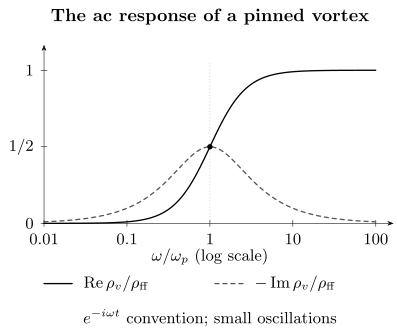
For $r=\omega/\omega_p$, the normalized dissipative part is $r^2/(1+r^2)$ and the plotted inductive magnitude is $r/(1+r^2)$. Their equality at $r=1$ marks equal restoring and viscous contributions. The result assumes small oscillations, negligible Hall response and no thermally activated escape.

What distinguishes a lattice, liquid or glass?

These labels concern different correlations and limits. They are not interchangeable descriptions of a hysteretic sample.

• An elastic solid has a shear response and extended positional correlations. One locally triangular image establishes only local order. Dislocations and finite resolution matter.
• A Bragg glass is a predicted weak-disorder elastic phase with algebraic translational correlations and no proliferated dislocations in the appropriate three-dimensional model. An experiment tests this asymptotic description over finite length scales; broadened peaks alone are insufficient.
• A vortex liquid lacks static shear rigidity, although it can have short-range order and a large viscosity. A thermodynamic melting claim requires equilibrium structural and thermodynamic support; a Lindemann displacement estimate is not a proof.
• A vortex glass requires a specified disorder model and controlled thermodynamic, long-time and small-current limits. Finite-window nonlinear curves and slow relaxation can mimic critical scaling.
• A Bose glass involves correlated line pinning and a distinct anisotropic response. Its name does not follow merely from the bosonic character of Cooper pairs.

Layering, finite thickness and line cutting can change which model applies. Equilibrium transitions also differ from dynamic reordering or heating-induced voltage jumps. At high drive, compare pulse duration, heat removal and local temperature before interpreting a discontinuity as intrinsic vortex dynamics.

Reading measurements together

Transport measures a voltage integrated between contacts. Field-sweep induction, current crowding and heating can accompany vortex motion. Magnetic susceptibility measures a history-dependent current distribution or small-signal response; a loop width alone does not identify microscopic pins.

Microwave measurements mix condensate, quasiparticle and vortex terms. Frequency dependence helps separate curvature from drag, but a single-frequency fit can be underdetermined. Tunneling images sample surface core spectra, while neutron scattering samples field modulation through the specimen. Peak loss can reflect domain size, mosaic spread, line wandering or motion during exposure as well as melting.

Comparison is most informative when temperature, internal induction, preparation and waiting time are matched. A probe with a $100\,\mathrm{nm}$ point-spread width cannot reliably resolve individual dislocations in a lattice spaced by $35\,\mathrm{nm}$; it may still reveal larger moving channels.

Example: a flux-flow estimate

Consider a hypothetical conventional film with $B=2.00\,\mathrm T$, $B_{c2}=20.0\,\mathrm T$ and $\rho_n=1.00\times10^{-6}\,\Omega\,\mathrm m$ at one temperature. A high-drive branch gives $\rho_{xx}=(1.02\pm0.05)\times10^{-7}\,\Omega\,\mathrm m$, consistent with the normal-core estimate $1.00\times10^{-7}\,\Omega\,\mathrm m$. Assume independent background analysis supports a vortex-channel interpretation and bounds $|\rho_{yx}/\rho_{xx}|<0.10$.

The longitudinal-only drag estimate is

$$\eta_0=\frac{B\Phi_0}{\rho_{xx}} \simeq4.06\times10^{-8}\,\mathrm{N\,s\,m^{-2}}.$$

Writing $r_H=\alpha_H/\eta=-\rho_{yx}/\rho_{xx}$ gives $\eta=\eta_0/(1+r_H^2)$, a correction below one percent. At $E_x=1.00\,\mathrm{V\,m^{-1}}$,

$$\begin{aligned} |v_y|&=E_x/B=0.500\,\mathrm{m\,s^{-1}},\\ J_x&\simeq9.80\times10^6\,\mathrm{A\,m^{-2}},\\ p&=J_xE_x\simeq9.80\times10^6\,\mathrm{W\,m^{-3}}. \end{aligned}$$

The inferred spacing is $a_0=34.6\,\mathrm{nm}$. Agreement of one slope does not prove homogeneous flow: matched imaging and pulse-temperature checks must test moving fractions and heating. Inferring $\xi=\sqrt{\Phi_0/(2\pi B_{c2})}$ far below $T_c$ would additionally require an orbital model valid there, rather than an automatic extrapolation of near-transition GL theory.

Exercises

1. Compression, shear and rigid rotation

For a wavevector along $x$, identify the in-plane displacement polarizations that probe compression and shear. Why is $u_x=-\Omega y$, $u_y=\Omega x$ a useful check on a real-space elastic formula?

Solution

A displacement along $x$ is longitudinal and probes $c_{11}$; one along $y$ is transverse and probes $c_{66}$. Variation along the vortex direction probes $c_{44}$. A rigid rotation has zero symmetrized strain, although $\partial_xu_y-\partial_yu_x=2\Omega$. Therefore a curl-squared density cannot be used alone as the finite-body shear energy. Bulk Fourier expressions rely on periodic modes or boundary terms treated consistently.

2. What does the relaxation energy measure?

At $30.0\,\mathrm K$, $|M_{\rm irr}|$ falls from $12.0$ to $10.2\,\mathrm{kA\,m^{-1}}$ between $10^2$ and $10^5\,\mathrm s$. Estimate $S$ and $U^\ast$. For the collective-creep model below, compare $U^\ast$ with $U$:

$$U(J)=\frac{U_c}{\mu} \left[\left(\frac{J_c}{J}\right)^\mu-1\right], \qquad \mu>0.$$

Solution

The finite-window logarithmic slope is $S=-\ln(10.2/12.0)/\ln(10^5/10^2)\simeq0.0235$. Thus $U^\ast=k_{\mathrm B}T/S\simeq110\,\mathrm{meV}$. Under the logarithmic-time approximation,

$$\begin{aligned} U^\ast&=-J U'(J) =U_c(J_c/J)^\mu,\\ &=U_c+\mu U(J). \end{aligned}$$

At $J=J_c$, the model barrier is zero but its logarithmic slope is $U_c$. The measured number is therefore not automatically a pin depth. Over a broad window it averages a changing rate; multiple barriers and changes in the current profile add further uncertainty.

3. Force, Hall sign and power

With $\mathbf J=J\hat{\mathbf x}$, $\mathbf B=B\hat{\mathbf z}$ and no pinning, solve the two-component force equation and verify positive dissipation.

Solution

The component equations are

$$\begin{aligned} \eta v_x-\alpha_Hv_y&=0,\\ \alpha_Hv_x+\eta v_y&=-J\Phi_0. \end{aligned}$$

They give $v_y=-J\Phi_0\eta/(\eta^2+\alpha_H^2)$ and $v_x=-J\Phi_0\alpha_H/(\eta^2+\alpha_H^2)$. Since $E_x=-Bv_y$ and $E_y=Bv_x$, the stated resistivity components follow. Finally,

$$\begin{aligned} J E_x&=\frac{B\Phi_0\eta J^2}{\eta^2+\alpha_H^2},\\ &=n_v\eta|\mathbf v|^2\ge0. \end{aligned}$$

The Hall term changes direction but supplies no dissipated power. Inverting only $\rho_{xx}$ gives $\eta_0=\eta(1+r_H^2)$, so neglecting a sizable Hall response overestimates drag in this model.

4. A pinning frequency without escape

Solve the harmonic pinning equation and show that $-\operatorname{Im}\rho_v/\operatorname{Re}\rho_v=\omega_p/\omega$. Does $\omega>\omega_p$ imply that vortices have left their wells?

Solution

The displacement amplitude is $u=\Phi_0J/(\alpha_p-i\omega\eta)$, and velocity is $-i\omega u$. Therefore, with $r=\omega/\omega_p$,

$$\begin{aligned} \frac{\operatorname{Re}\rho_v}{\rho_{\rm ff}}&=\frac{r^2}{1+r^2},\\ \frac{-\operatorname{Im}\rho_v}{\rho_{\rm ff}}&=\frac{r}{1+r^2}. \end{aligned}$$

Their ratio is $1/r$. The displacement magnitude actually decreases with frequency at fixed force amplitude. The high-frequency resistive limit can therefore occur while motion remains inside a harmonic well. Escape requires information about the nonlinear potential, drive amplitude and thermal activation.

5. A broadened peak and a voltage onset

A magnetic loop opens, transport becomes nonlinear and an image shows sixfold local coordination below $T_\star$. What is established, and what additional observations could distinguish melting from pinning?

Solution

The observations establish a correlated vortex configuration with history-dependent response on the measured scales. They do not uniquely establish a lattice, liquid or glass transition. Spatial correlation and dislocation measurements test extended order; reversible calorimetry or magnetization can test a thermodynamic change; waiting-time, drive and sample-size dependence test dynamic freezing and creep. Structural and transport measurements should use matched histories. A finite nonlinear curve alone cannot supply the thermodynamic and zero-current limits of a glass claim.

References

• P. W. Anderson and Y. B. Kim, “Hard Superconductivity: Theory of the Motion of Abrikosov Flux Lines,” Reviews of Modern Physics 36, 39–43 (1964), doi:10.1103/RevModPhys.36.39.
• J. Bardeen and M. J. Stephen, “Theory of the Motion of Vortices in Superconductors,” Physical Review 140, A1197–A1207 (1965), doi:10.1103/PhysRev.140.A1197.
• C. P. Bean, “Magnetization of Hard Superconductors,” Physical Review Letters 8, 250–253 (1962), doi:10.1103/PhysRevLett.8.250.
• C. P. Bean and J. D. Livingston, “Surface Barrier in Type-II Superconductors,” Physical Review Letters 12, 14–16 (1964), doi:10.1103/PhysRevLett.12.14.
• G. Blatter, M. V. Feigel’man, V. B. Geshkenbein, A. I. Larkin, and V. M. Vinokur, “Vortices in High-Temperature Superconductors,” Reviews of Modern Physics 66, 1125–1388 (1994), doi:10.1103/RevModPhys.66.1125.
• E. H. Brandt, “The Flux-Line Lattice in Superconductors,” Reports on Progress in Physics 58, 1465–1594 (1995), doi:10.1088/0034-4885/58/11/003.
• A. M. Campbell, “The Response of Pinned Flux Vortices to Low-Frequency Fields,” Journal of Physics C: Solid State Physics 2, 1492–1501 (1969), doi:10.1088/0022-3719/2/8/318.
• D. S. Fisher, M. P. A. Fisher, and D. A. Huse, “Thermal Fluctuations, Quenched Disorder, Phase Transitions, and Transport in Type-II Superconductors,” Physical Review B 43, 130–159 (1991), doi:10.1103/PhysRevB.43.130.
• T. Giamarchi and P. Le Doussal, “Elastic Theory of Pinned Flux Lattices,” Physical Review Letters 72, 1530–1533 (1994), doi:10.1103/PhysRevLett.72.1530.
• J. I. Gittleman and B. Rosenblum, “Radio-Frequency Resistance in the Mixed State for Subcritical Currents,” Physical Review Letters 16, 734–736 (1966), doi:10.1103/PhysRevLett.16.734.
• A. I. Larkin and Yu. N. Ovchinnikov, “Pinning in Type II Superconductors,” Journal of Low Temperature Physics 34, 409–428 (1979), doi:10.1007/BF00117160.
• Y. Yeshurun, A. P. Malozemoff, and A. Shaulov, “Magnetic Relaxation in High-Temperature Superconductors,” Reviews of Modern Physics 68, 911–949 (1996), doi:10.1103/RevModPhys.68.911.