Disorder in Quantum Matter

Disorder is a spatial or temporal variation of the parameters that govern quantum motion. A missing atom, a rough interface and a fluctuating charge trap can all change an electron’s potential, but they scatter different momenta and act on different timescales. Describing disorder therefore requires both a Hamiltonian and a probability distribution for its varying parameters.

The central example on this page is smooth scalar disorder: it can scatter a particle many times while barely changing the direction of its current. This explains why a spectral linewidth, a mobility and a phase-coherence time measure different properties. Anderson localization develops the subsequent buildup of coherent multiple scattering.

Required background. Conventions for Quantum Matter supplies charge and spectral conventions. Boltzmann Transport explains the collision operator and current relaxation; the First Born Approximation explains weak-potential scattering.

Random terms in a Hamiltonian

For an electron in a microscopic periodic potential, start with $p^2/(2m_e)+V_{\mathrm{per}}(\mathbf r)$. After projecting into a nondegenerate band near a parabolic extremum, a different, approximate description is

$$H_{\mathrm{env}}=\frac{\mathbf p^2}{2m^*}+U(\mathbf r).$$

Here the effective mass already incorporates the clean crystal’s band curvature. Adding the original microscopic periodic potential to this projected Hamiltonian would count that band structure twice. The scalar envelope description assumes that neglected bands and internal wavefunction structure do not appreciably alter the scattering; smooth disorder helps justify that assumption.

On a lattice, an elementary model instead uses

$$\begin{aligned} H&=\sum_i\epsilon_i c_i^\dagger c_i+H_t,\\ H_t&=-\sum_{\langle ij\rangle} \left(t_{ij}c_i^\dagger c_j+\mathrm{h.c.}\right). \end{aligned}$$

Random site energies $\epsilon_i$ are diagonal disorder; random hopping amplitudes $t_{ij}$ are bond disorder. The on-site Anderson model holds hopping fixed and randomizes site energies, isolating a mechanism rather than representing every disordered material (Anderson, 1958).

Physical variation	Possible model change
Substitution or a trapped charge	Local potential, carrier density or screening
Vacancy or a damaged bond	Removed orbital, altered hopping or local moment
Interface roughness or strain	Confinement energy and spatially correlated hopping
Frozen magnetic moments	A random exchange term $\mathbf h_i\cdot\boldsymbol\sigma$
Moving traps or ions	A time-dependent potential and its noise spectrum

One defect can produce several of these changes. A random magnetic field with zero mean can still break time reversal in every sample. Likewise, a translation-invariant disorder distribution does not give one random sample exact Bloch momentum. Elliott, Krumhansl and Leath (1974) develop this distinction between microscopic randomness and averaged descriptions.

Frozen, equilibrating and fluctuating variables

Quenched disorder is fixed during the evolution and measurement. Calculate the observable at fixed $U$, then average over realizations. Annealed variables equilibrate together with the matter: their configurations belong inside the partition sum. For a specified normalized bare distribution $P(U)$, the corresponding free-energy expressions are

$$\begin{aligned} F_{\mathrm q}&=-k_BT\,\overline{\ln Z_U},\\ F_{\mathrm a}&=-k_BT\ln\overline{Z_U}. \end{aligned}$$

The overline uses the same $P(U)$ in both expressions. In a physical annealed model, the energy and entropy of the varying variables must be included in that bare weight; its normalization contributes a reference free energy. The coupled annealed distribution is proportional to $P(U)Z_U$, not generally $P(U)$.

Dynamic disorder fluctuates on the observation timescale and can exchange energy or cause dephasing. The same trap can look frozen during a short pulse but fluctuate during a long trace. “Annealed” therefore means equilibration, not simply “time dependent.”

Spatial correlations select momentum transfers

For statistically homogeneous scalar disorder, subtract its constant mean and define

$$\begin{aligned} \delta U(\mathbf r)&=U(\mathbf r)-\overline U,\\ C(\mathbf r-\mathbf r')&= \overline{\delta U(\mathbf r)\delta U(\mathbf r')}. \end{aligned}$$

The Fourier convention and power spectrum are

$$\begin{aligned} U_{\mathbf q}&=\int d^dr\,e^{-i\mathbf q\cdot\mathbf r}\delta U(\mathbf r),\\ S_U(\mathbf q)&=\int d^dr\,e^{-i\mathbf q\cdot\mathbf r}C(\mathbf r). \end{aligned}$$

In an infinite homogeneous ensemble,

$$\overline{U_{\mathbf q}U_{\mathbf q'}} =(2\pi)^d\delta^{(d)}(\mathbf q+\mathbf q') \times S_U(\mathbf q).$$

The plus sign in the delta function appears because neither Fourier amplitude is conjugated. For a real potential, $U_{-\mathbf q}=U_{\mathbf q}^*$. The spectrum has units of energy squared times length to the power $d$ and is nonnegative. Plane waves normalized in a large volume $\mathcal V$ have averaged squared scattering matrix element $S_U(\mathbf k'-\mathbf k)/\mathcal V$.

For a Gaussian spatial correlation,

$$\begin{aligned} C(r)&=W^2e^{-r^2/(2\xi_d^2)},\\ S_U(q)&=(2\pi)^{d/2}W^2\xi_d^d e^{-q^2\xi_d^2/2}. \end{aligned}$$

Here $W$ is the root-mean-square potential and $\xi_d$ is its correlation length. Increasing $\xi_d$ narrows the momentum-transfer spectrum. This Gaussian shape of the covariance need not imply that the random field has Gaussian statistics. Only for a Gaussian random field do the mean and covariance determine every higher moment.

White noise, $C(\mathbf r)=\gamma\delta^{(d)}(\mathbf r)$, has constant spectrum $S_U=\gamma$. It needs a physical cutoff for quantities sensitive to arbitrarily short distances. Taking $\xi_d\to0$ at fixed $W$ in the preceding smooth model gives vanishing integrated covariance; to approach white noise with fixed $\gamma$, keep $(2\pi)^{d/2}W^2\xi_d^d=\gamma$ instead. Quoting a “disorder strength” without its convention can obscure this distinction.

For independently placed dilute impurities of profile $u(\mathbf r)$ and density $n_i$, the connected spectrum is $S_U(q)=n_i|u_{\mathbf q}|^2$, away from the mean-potential contribution. Correlations among impurity positions introduce a structure factor. Changing density and changing the impurity profile are therefore different interventions.

Spectral scattering and current relaxation

Assume weak elastic scattering in one isotropic scalar band. With $\mathbf q=\mathbf k'-\mathbf k$, define the final-state measure

$$d\Pi_{\mathbf k'}= \frac{d^dk'}{(2\pi)^d}\, \delta(\epsilon_{\mathbf k'}-\epsilon_{\mathbf k}).$$

The differential Born scattering rate is $d\Gamma=(2\pi/\hbar)S_U(\mathbf q)\,d\Pi_{\mathbf k'}$. The two lifetimes follow by integrating it with different weights:

$$\begin{aligned} \tau_q^{-1}&=\int d\Gamma,\\ \tau_{\mathrm{tr}}^{-1}&=\int(1-\cos\theta)\,d\Gamma. \end{aligned}$$

Every allowed scattering event contributes to the quantum rate. Current relaxation instead weights how much forward velocity is lost: a small deflection has $1-\cos\theta\simeq\theta^2/2$. This angular factor follows from the first angular harmonic of the isotropic collision operator. An anisotropic or multiband problem requires solving that operator with the appropriate velocity and wavefunction matrix elements.

In the weak, nearly energy-independent self-energy approximation,

$$\begin{aligned} \overline{G^R(\mathbf k,E)}&= \frac{1}{E-\epsilon_{\mathbf k}-\Sigma^R},\\ \operatorname{Im}\Sigma^R&=-\frac{\hbar}{2\tau_q}. \end{aligned}$$

The spectral Lorentzian has full width $\hbar/\tau_q$. Energy-dependent self-energy, quasiparticle weight, interaction broadening and instrumental resolution can change that inference; see spectral functions. Mobility instead gives $\mu=e\tau_{\mathrm{tr}}/m^*$ in the one-band Drude model.

A calculable smooth-disorder example

On a two-dimensional circular Fermi surface, $q=2k_F\sin(\theta/2)$. For the Gaussian covariance, put $a=k_F\xi_d$. The angular scattering rate is proportional to

$$w(\theta)\propto e^{-a^2(1-\cos\theta)}.$$

Thus

$$\frac{\tau_{\mathrm{tr}}}{\tau_q} =\frac{\int_0^{2\pi} w(\theta)\,d\theta} {\int_0^{2\pi}w(\theta)(1-\cos\theta)\,d\theta}.$$

For $a\ll1$, scattering is nearly isotropic and the ratio tends to one. For $a\gg1$, typical deflections are of order $1/a$ and the ratio approaches $2a^2$. At $a=2$, direct integration gives 7.33.

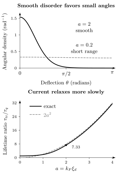
Top: angular distributions normalized to the same total scattering probability, with deflection angles folded onto $0\le\theta\le\pi$. Smooth disorder favors small deflections. Bottom: their different angular weighting makes the lifetime ratio grow; the dashed curve is the large-$a$ approximation $2a^2$. Absolute rates also depend on the disorder amplitude. These curves describe a scalar parabolic band without an additional spinor overlap.

A lifetime ratio is a clue to angular structure, not a unique reconstruction of the defects. In graphene, even a momentum-independent scalar potential has a spinor overlap that suppresses backscattering. Hwang and Das Sarma (2008) show why graphene and ordinary two-dimensional electron gases need different lifetime calculations.

Scattering does not itself erase coherence

A static Hermitian random Hamiltonian preserves purity within each isolated realization. Averaging over unknown realizations can nevertheless reduce ensemble coherence, as Exercise 3 shows. This distinction underlies coherent interference corrections in disordered conductors (Lee and Ramakrishnan, 1985).

At an isotropic Fermi surface,

$$\begin{aligned} \ell_q&=v_F\tau_q,\\ \ell_{\mathrm{tr}}&=v_F\tau_{\mathrm{tr}},\\ D&=v_F^2\tau_{\mathrm{tr}}/d,\\ L_\phi&=\sqrt{D\tau_\phi}. \end{aligned}$$

The diffusion formulas apply after angular relaxation. For a system with localization length $\xi$, a coherent diffusive window requires $\ell_{\mathrm{tr}}\ll L\ll\xi$ and $L\lesssim L_\phi$. Having $L>\ell_{\mathrm{tr}}$ alone does not establish diffusion. In a metallic regime, no finite localization length cuts off that diffusion.

Likewise, $k_F\ell_{\mathrm{tr}}\gg1$ does not by itself guarantee a narrow quasiparticle peak when forward scattering makes $\tau_q\ll\tau_{\mathrm{tr}}$. Check the quantum broadening against the relevant band scales and the validity of the Born approximation separately. A wavelength comparable to a mean free path signals the failure of a simple semiclassical picture, not a universal transition criterion. Quantum coherence in conductors separates dephasing, escape and thermal averaging.

Comparing models with measurements

An observable is generally nonlinear in the random potential: $\overline{X[U]}\ne X[\overline U]$. An averaged one-particle Green function can describe a mean spectrum, while conductivity requires correlated propagation and appropriate vertex corrections. A self-energy alone is not automatically a transport calculation.

Measurement	What must be distinguished
Mobility or residual resistivity	Momentum relaxation, carrier density and band parameters
Dingle damping or spectral linewidth	Quantum broadening, other damping and resolution
Local tunneling spectrum	Local density of states versus the bare potential
Diffuse scattering or microscopy	Structural correlations and the sampled field of view
Time traces and noise	Dynamic fluctuators versus frozen disorder

State what constitutes the ensemble: different samples, spatial regions, or a parameter sweep. A magnetic-field sweep changes interference phases without necessarily moving defects. Thermal cycling can alter contacts as well as disorder. Broad distributions and rare events may prevent an arithmetic mean from representing a typical sample; universal conductance fluctuations discusses this experimentally.

Changing a dopant fraction can change density, strain and interactions together with randomness. To isolate a disorder effect, compare the relevant quantities independently. Disorder can pin vortices, alter superconducting proximity, or create localized states supporting Hall plateaus. The outcome depends on how the disorder couples to the states and symmetries, rather than on a universal amount of “dirtiness.” Computational Quantum Matter helps choose the corresponding numerical method.

Exercises

1. Same variance, different statistics

For a binary alloy with site energies $V_A,V_B$ and probabilities $p,1-p$, find the mean and variance. At $p=1/2$ with $V_A=W$, $V_B=-W$, compare its fourth moment with a zero-mean Gaussian of variance $W^2$.

Solution

The mean is $pV_A+(1-p)V_B$ and the variance is $p(1-p)(V_A-V_B)^2$. For the symmetric alloy, $\overline{\epsilon^4}=W^4$, whereas the Gaussian gives $3W^4$. The connected fourth moment is therefore $-2W^4$ for the binary distribution and zero for the Gaussian. A covariance alone does not determine non-Gaussian tails or higher-order scattering statistics.

2. The smooth-scattering limit

Explain the ratio $\tau_{\mathrm{tr}}/\tau_q\simeq2a^2$ for $a=k_F\xi_d\gg1$ without using special functions. Does the approximation give the exact ratio at $a=2$?

Solution

Near forward scattering, the angular distribution is proportional to $e^{-a^2\theta^2/2}$. Extending the narrow peak to the real line gives $\langle\theta^2\rangle=1/a^2$. Consequently,

$$\frac{\tau_q}{\tau_{\mathrm{tr}}} =\langle1-\cos\theta\rangle \simeq\frac{1}{2a^2}.$$

At $a=2$ the approximation gives 8, compared with the exact angular integral 7.33. Its error is about 9%; the condition $a\gg1$ matters. The full crossover is plotted above.

3. Static randomness and a spin echo

Each run evolves a spin initially in $|+x\rangle$ under $H_\pm=\pm\hbar\Omega\sigma_z/2$, with equal probabilities and a fixed sign during the run. Find the purity of the averaged state. What does an ideal $\pi$ pulse about $x$ halfway through the evolution do?

Solution

The two pure states rotate in opposite directions, giving

$$\begin{aligned} \overline\rho(t)&=\tfrac12[I+\cos(\Omega t)\sigma_x],\\ \operatorname{Tr}\overline\rho^{\,2} &=\tfrac12[1+\cos^2(\Omega t)]. \end{aligned}$$

At $\Omega t=\pi/2$ the mixture is maximally mixed, although each run remains pure. Because $\sigma_x H_\pm\sigma_x=-H_\pm$, the second half reverses the first half’s phase accumulation. The spin returns to $|+x\rangle$ up to a phase in both realizations. Fluctuations during the sequence, other Hamiltonian terms or imperfect pulses can spoil this refocusing.

4. A mean free path from mobility

A spin-degenerate circular two-dimensional band has density $3.0\times10^{11}\,\mathrm{cm}^{-2}$ and mobility $10^6\,\mathrm{cm}^2/(\mathrm{V\,s})$. Find $k_F$, $\ell_{\mathrm{tr}}$ and their product. Does this determine $\tau_q$?

Solution

In SI units, $n=3.0\times10^{15}\,\mathrm{m}^{-2}$ and $\mu=100\,\mathrm{m}^2/(\mathrm{V\,s})$. Counting both spin states gives

$$k_F=\sqrt{2\pi n}\simeq1.37\times10^8\,\mathrm{m}^{-1}.$$

Combining $v_F=\hbar k_F/m^*$ and $\tau_{\mathrm{tr}}=m^*\mu/e$ gives

$$\begin{aligned} \ell_{\mathrm{tr}}&=\hbar k_F\mu/e\simeq9.04\,\mu\mathrm m,\\ k_F\ell_{\mathrm{tr}}&\simeq1.24\times10^3. \end{aligned}$$

The mass cancels in this one-band result. The quantum lifetime remains undetermined without the angular scattering spectrum or an independent spectral measurement. Other degeneracies or multiple conducting bands change the inference.

5. Quenched and annealed averages

Two environments have equal bare probability and partition functions $Z_1=1$, $Z_2=9$. Find $F_{\mathrm q}/(k_BT)$, $F_{\mathrm a}/(k_BT)$ and the annealed probabilities. Verify the ordering using Jensen’s inequality.

Solution

The quenched expression is $-\tfrac12\ln9=-\ln3$, while the annealed expression is $-\ln5$. Annealed weights are proportional to $(1/2,9/2)$, hence probabilities $(0.1,0.9)$. The environment with more accessible matter states is favored when it can equilibrate.

Since the logarithm is concave, $\overline{\ln Z}\le\ln\overline Z$. Multiplying by $-k_BT$ gives $F_{\mathrm q}\ge F_{\mathrm a}$. The comparison uses the same bare distribution and free-energy reference for both models.

References

• P. W. Anderson, “Absence of Diffusion in Certain Random Lattices,” Physical Review 109, 1492–1505 (1958), doi:10.1103/PhysRev.109.1492.
• R. J. Elliott, J. A. Krumhansl, and P. L. Leath, “The Theory and Properties of Randomly Disordered Crystals and Related Physical Systems,” Reviews of Modern Physics 46, 465–543 (1974), doi:10.1103/RevModPhys.46.465.
• E. H. Hwang and S. Das Sarma, “Single-Particle Relaxation Time versus Transport Scattering Time in a Two-Dimensional Graphene Layer,” Physical Review B 77, 195412 (2008), doi:10.1103/PhysRevB.77.195412.
• P. A. Lee and T. V. Ramakrishnan, “Disordered Electronic Systems,” Reviews of Modern Physics 57, 287–337 (1985), doi:10.1103/RevModPhys.57.287.