Mobility Edges

A mobility edge is an energy at which the thermodynamic character of single-particle states changes between localized and extended. The density of states need not vanish there. What changes is the ability of states in an arbitrarily narrow energy window to carry amplitude, particles, or waves across arbitrarily large distances.

This definition is intrinsically scale-dependent. Every eigenstate of a finite closed sample is normalizable, and a large localization length can exceed every simulated or experimental dimension. A mobility-edge claim therefore requires energy-resolved finite-size, finite-time, or finite-frequency scaling. A sharp-looking change in one finite sample is suggestive, not yet an edge in the thermodynamic sense.

Here the focus is a noninteracting, coherent system: how an energy scan crosses a localization transition, and how finite resolution changes what we observe. A single-particle mobility edge does not by itself imply a many-body mobility edge.

Required background. Anderson Localization supplies the distinctions among localized eigenstates, bounded spreading and suppressed transmission. Scaling Theory of Localization supplies finite-size flow and critical localization-length scaling, needed to distinguish a mobility edge from a finite-resolution crossover.

Spectral boundaries between localized and extended states

Specify the disorder distribution, spatial correlations, symmetry class and energy zero before comparing edge positions. The main example below is the three-dimensional orthogonal Anderson model. Its edge location depends on these microscopic choices; its critical exponents can be shared by other models in the same universality class.

Spectral support and mobility are different

Let

$$\rho(E) = \frac{1}{V} \sum_\alpha \delta(E-E_\alpha)$$

be the single-particle density of states per volume. It answers whether eigenvalues occur near $E$. It does not answer how those eigenstates scale in space.

For an energy-filtered wave packet, define the mean-square displacement

$$\Delta r_E^2(t) = \left\langle \lvert \mathbf r(t)-\mathbf r(0) \rvert^2 \right\rangle_E.$$

In a diffusive extended regime,

$$\Delta r_E^2(t) \sim 2dD(E)t,$$

whereas a packet confined to an energy interval with dynamical localization has bounded spreading. It may keep fluctuating rather than converge to an exact plateau. Its spatial extent depends on both its preparation and the localization lengths in that interval; $\xi^2$ gives a characteristic spreading scale, not a universal final variance. The interval must stay away from the edge for its largest localization length to remain finite.

The corresponding energy-resolved diffusion constant is

$$D(E) = \lim_{t\to\infty} \frac{ \Delta r_E^2(t) }{ 2dt }.$$

At a conventional continuous three-dimensional transition with a finite density of states, $D(E)=0$ on the localized side and $D(E)>0$ in the diffusive metal. For a lower edge of the extended band,

$$\rho(E_c)>0,\qquad \lim_{E\downarrow E_c}D(E)=0.$$

The diffusion constant approaches zero continuously from the metal. At criticality, spreading can still grow subdiffusively even though the long-time diffusion constant vanishes. Thus zero $D$ alone does not distinguish a localized state from the critical state.

Boundary or interval	What it means
Spectral band edge	No eigenstates occur beyond the spectral support.
Mobility edge	States change their spatial scaling; the density of states can stay smooth.
Spectral gap	An interval contains no bulk single-particle states.
Mobility gap	An interval contains no extended bulk states; localized states can remain.

A mobility gap is an interval without extended bulk states. A mobility edge is one boundary of such an interval. The two terms are related but not interchangeable.

An energy-resolved statement

A mobility edge is not a single label attached to the whole Hamiltonian. One model can have:

• localized lower and upper spectral tails surrounding an extended central band;
• several extended windows separated by localized windows;
• only isolated critical energies, as in idealized quantum Hall scaling;
• no mobility edge because all states are localized;
• no localized states in the energy range under study.

The edge can move when disorder strength, correlation length, magnetic field, spin–orbit coupling, lattice geometry, or quasiperiodic structure changes. Correlated disorder can even create special transparent energies. These are model properties, not exceptions to the definition.

Dimension and symmetry matter. Ordinary short-range, uncorrelated disorder localizes the generic one-dimensional orthogonal model; a topologically trivial two-dimensional orthogonal model also flows toward localization. Spin–orbit coupling, topology and special correlations can change that conclusion. See Anderson Localization for the distinctions among these settings.

Chemical potential and temperature

For electrons, a mobility edge matters to dc transport only after its position is compared with the chemical potential. If extended states begin at $E_c>\mu$, define

$$\Delta_{\mathrm{mob}} = E_c-\mu > 0.$$

Thermal excitation into extended states can produce

$$\sigma_{\mathrm{ext}}(T) \sim \sigma_a(T) \exp\!\left( -\frac{ \Delta_{\mathrm{mob}} }{ k_{\mathrm B}T } \right).$$

Localized states near $\mu$ can simultaneously conduct by bath-assisted hopping. When the two mechanisms act as parallel channels, their conductivities add; the larger contribution controls the observed temperature dependence.

An Arrhenius slope can be compatible with activation to a mobility edge, but it does not prove that interpretation. A hard band gap, contact barrier, nearest-neighbor hop, or polaron activation can produce the same exponent.

Finite temperature also introduces an inelastic length $L_\phi(T)$ and an energy window. A measured response has the schematic form

$$\mathcal O_{\mathrm{meas}} = \int dE\, K(E;\mu,T,\Delta E) \mathcal O(E),$$

where $K$ contains occupation, instrumental resolution, and preparation effects. If the kernel straddles $E_c$, the observed crossover is rounded even for an ideal sharp zero-temperature edge.

Three-dimensional localization

The simple-cubic benchmark

Consider the nearest-neighbor simple-cubic Anderson model defined on Anderson Localization, with hopping $t$ and independent site energies uniformly distributed over

$$\varepsilon_i \in \left[ -\frac{W}{2}, \frac{W}{2} \right].$$

At $W=0$, the clean dispersion is

$$E(\mathbf k)=-2t\sum_{j=x,y,z}\cos(k_ja),$$

so the clean band occupies

$$-6t \le E \le 6t.$$

Weak disorder broadens the spectrum and creates localized tail states while an extended core survives. At a fixed $W$, scanning energy can cross a lower mobility edge into the extended core and an upper edge back into localized states. Increasing disorder eventually removes the extended window.

For box disorder at $E=t$, Slevin and Ohtsuki (2014, Tables 3–4) find approximately

$$\frac{W_c}{t} \simeq 16.53.$$

This is not a material constant and not a universal number. It belongs to this lattice, hopping convention, site-energy distribution, energy, and orthogonal symmetry class.

Near a clean spectral edge, disorder can both localize states and mix otherwise off-resonant sites. The mobility-edge curve can therefore bend nonmonotonically before the extended region finally collapses. This reentrant shape is a property of the model phase diagram; it should not be inferred from a monotonic “more disorder means lower mobility” slogan.

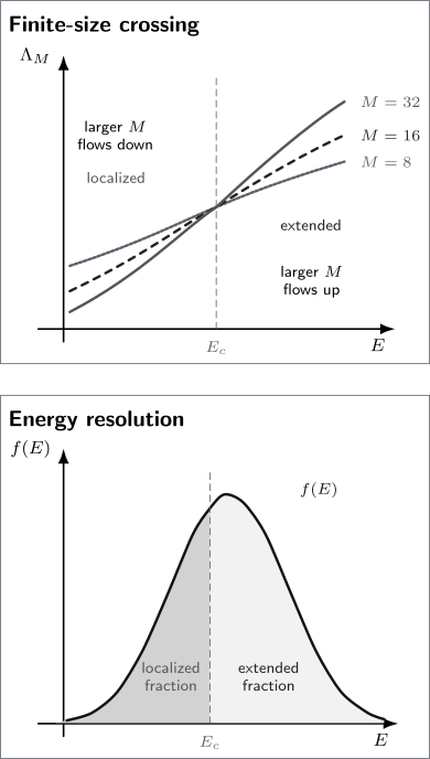
Two ways to resolve an edge. Top: schematic transfer-matrix curves cross when the dimensionless localization length becomes independent of bar width; corrections can shift the crossings in actual data. Bottom: an illustrative energy distribution straddles a lower edge of an extended band. The areas on either side give localized and extended fractions, even when the distribution’s peak is above the edge. Neither panel is a numerical phase diagram.

Why three dimensions permit the transition

For a hypercubic conductor with bulk conductivity $\sigma$, the dimensionless conductance scales classically as

$$g(L) \sim \frac{ \sigma L^{d-2} }{ e^2/h }.$$

The geometric factor grows with $L$ in $d=3$, while localization corrections reduce conductance. Their competition permits an unstable critical point. On one side, the flow approaches a metal; on the other, it approaches exponentially small conductance.

This argument explains why a transition is possible, not where $E_c(W)$ lies. The edge location requires microscopic calculation or measurement. Spatial correlations in a laser speckle, long-range hopping, anisotropy, multiple orbitals, and magnetic fields can shift the edge strongly without changing every universal exponent.

Disorder broadening is not delocalization

The operator spectrum for bounded box disorder lies within the broad bound

$$-6t-\frac{W}{2} \le E \le 6t+\frac{W}{2}.$$

This growing spectral support does not imply a growing extended band. Disorder can add localized tail states while the extended region shrinks. A density-of-states plot can therefore broaden at the same time that the mobility window narrows.

That distinction is especially important in amorphous semiconductors and impurity bands. A spectroscopic onset locates available states; a transport onset locates states that participate in long-range motion under the stated conditions. Their separation is a mobility-tail regime, not automatically a clean band gap.

Critical behavior

Diverging length

Choose a dimensionless tuning variable $\delta$ with $\delta=0$ at the edge and $\delta>0$ on the extended side. For an energy scan at fixed disorder, one convenient local definition is

$$\delta = \frac{ E-E_c }{ E_0 },$$

with the sign reversed at an upper edge if needed. The critical length diverges as

$$\xi_\pm(\delta) = \xi_{0,\pm} \lvert\delta\rvert^{-\nu}.$$

On the localized side, $\xi_-$ is the localization length. On the metallic side, $\xi_+$ is a correlation or crossover length beyond which metallic scaling is established. The amplitudes $\xi_{0,+}$ and $\xi_{0,-}$ need not be equal.

For the three-dimensional orthogonal class, Slevin and Ohtsuki (2014, Table 5) report

$$\nu \simeq 1.571,$$

with a reported interval approximately

$$1.563 \le \nu \le 1.579.$$

This is a numerical estimate of a universal exponent, with a reported 95% confidence interval for that analysis. It is not an exact value or an uncertainty assigned to every method. Edge locations and length amplitudes are nonuniversal. A critical conductance distribution can have universal features within fixed geometry and boundary conventions, but changing those conventions can change the distribution (Evers and Mirlin, 2008).

For a broad class of random systems satisfying the assumptions of Chayes et al. (1986), including suitable short-range disorder, the finite-size correlation-length exponent obeys

$$\nu_{\mathrm{FS}} \ge \frac{2}{d}.$$

The three-dimensional orthogonal value comfortably satisfies this bound. An apparent violation calls for checking the theorem’s assumptions, available sizes and crossover scales, and whether the fitted length is the finite-size correlation length.

Conductivity exponent

On the metallic side at zero temperature,

$$\sigma(\delta,0) \propto \delta^s.$$

Under noninteracting one-parameter scaling with a finite nonsingular density of states, the Wegner relation gives

$$s = (d-2)\nu.$$

Thus in three dimensions,

$$s = \nu.$$

This relation is not a license to fit an interacting finite-temperature material with one exponent. Electron–electron interactions, changing carrier density, finite $L_\phi$, and inhomogeneity can introduce extra scaling variables and alter the transport analysis.

At criticality, the finite-sample conductance can be scale-invariant while the bulk conductivity behaves as

$$\sigma(L) \sim \frac{e^2}{h} L^{2-d}.$$

In $d=3$, the thermodynamic dc conductivity at the critical point therefore vanishes even though the finite-size dimensionless conductance remains of order unity.

Dynamical scaling

A frequency or observation time supplies a finite length,

$$L_\omega \sim \omega^{-1/z}.$$

For the standard noninteracting Anderson transition with a regular density of states, the dynamical exponent is

$$z=d.$$

The critical ac conductivity then scales as

$$\operatorname{Re}\sigma(\omega,E_c) \propto \omega^{(d-2)/d},$$

so the three-dimensional benchmark is

$$\operatorname{Re}\sigma(\omega,E_c) \propto \omega^{1/3}.$$

These frequency laws assume the thermodynamic limit before the zero-frequency limit and a noninteracting system with a regular density of states. A finite isolated sample instead has discrete absorption lines. Temperature, interactions and coupling to a probe can introduce further scales.

Critical eigenstates are multifractal

Critical states are neither uniformly extended nor exponentially localized. For lattice probabilities

$$\mu_i = \lvert\psi_i\rvert^2,$$

define generalized participation moments

$$P_q = \sum_i \mu_i^q.$$

Measuring $L$ in lattice spacings, at criticality

$$P_q \propto L^{-\tau_q},$$

with

$$\tau_q = d(q-1) + \Delta_q.$$

The anomalous exponents $\Delta_q$ vanish for a perfectly uniform extended state but are nonzero at an Anderson critical point. For $q=2$,

$$P_2 \propto L^{-D_2}, \qquad 0<D_2<d.$$

Multifractality is a distributional statement over scales and disorder realizations. A single visually sparse eigenfunction is not a multifractal analysis.

Finite-size identification

Transfer-matrix crossing

For a long bar with transverse width $M$, let $\lambda_M(E)$ be the quasi-one-dimensional localization length obtained from the smallest positive Lyapunov exponent. The dimensionless ratio

$$\Lambda_M(E) = \frac{ \lambda_M(E) }{ M }$$

decreases with increasing width in the localized regime and increases in the extended regime. At the critical point it approaches a width-independent value. This reverses the finite-size trend without requiring a visual classification of individual eigenfunctions (MacKinnon and Kramer, 1981).

Near the edge, a precision fit uses both relevant and irrelevant scaling fields:

$$\Lambda_M = \mathcal F \left( \chi(\delta)M^{1/\nu}, \phi(\delta)M^y \right).$$

Here $y<0$, and $M$ is expressed in lattice units. The irrelevant term explains why crossings of successive widths drift rather than meeting at one perfect point. If corrections are negligible, the critical slope obeys

$$\left. \frac{ \partial\Lambda_M }{ \partial E } \right|_{E_c} \propto M^{1/\nu}.$$

One crossing of two widths estimates a crossover. A reliable fit tests its sensitivity to the minimum width, energy window and irrelevant corrections, with enough independent disorder samples to estimate uncertainty. Finite-Size Scaling in Numerics explains how to fit correlated data.

Complementary observables

Observable	What to compare as size grows
Transfer length $\Lambda_M$	Decreasing and increasing flows on opposite sides.
Participation moments	Localized saturation, extended volume scaling and critical anomalous powers.
Conductance	Its distribution and size dependence, with fixed contacts and geometry.
Wave-packet spreading	Bounded expansion, diffusion or critical subdiffusion over longer times.
Level statistics	Energy-resolved distributions after resolving symmetries.

These observables probe different aspects of the same states. Level statistics require special care with unresolved symmetry sectors and degeneracies.

Energy binning can mix the two phases. If eigenstates in a bin $\mathcal B$ are pooled with equal weight per state, their mean observable is

$$\overline{\mathcal O}_{\mathcal B} =\frac{\int_{\mathcal B}\rho(E)\mathcal O(E)\,dE} {\int_{\mathcal B}\rho(E)\,dE}.$$

The density of states appears because an energy interval containing more states contributes more samples. A uniform average on an energy grid uses a different weight. Shrinking and shifting the bin tests whether an apparent intermediate exponent comes from critical states or from mixing localized and extended ones.

Experimental probes

Electronic materials

In a disordered solid, carrier density, gate voltage, pressure, composition or magnetic field are more accessible controls than eigenenergy itself. They can change the chemical potential together with disorder screening, interactions, band structure and inelastic scattering.

A density-tuned metal–insulator transition is therefore not automatically a clean scan of $\mu$ through a fixed single-particle $E_c$. The microscopic ensemble must remain sufficiently controlled for that interpretation.

Thermal activation is more convincing when its fitted energy agrees with an independently determined offset from the chemical potential. If hopping dominates, compare the localization length, density of states and dielectric scale using Anderson Insulators. Tunneling and photoemission locate spectral weight, which alone does not determine mobility. The local density-of-states distribution adds spatial information, provided size and energy broadening are scaled together.

Ultracold atoms

Cold atoms offer unusually direct control over disorder and dynamics. A typical protocol prepares a normalized energy distribution $f(E)$, releases the cloud into a three-dimensional random potential, and tracks expansion. If localized states lie below $E_c$, the ideal localized fraction is

$$f_{\mathrm{loc}} = \int_{-\infty}^{E_c} dE\, f(E).$$

The extended fraction is

$$f_{\mathrm{ext}} = 1-f_{\mathrm{loc}}.$$

This makes energy calibration central. An uncertainty in $f(E)$ or the zero of the speckle potential maps directly into uncertainty in $E_c$. Residual interactions, finite observation time, trap curvature, anisotropic speckle correlations, and classical trapping below a percolation threshold must be controlled.

Diffusion increases the mean-square displacement linearly with time, whereas dynamical localization keeps the expansion bounded. Classical trapping can also produce a stationary cloud, so a stationary image alone cannot identify the quantum mechanism.

Semeghini et al. (2015) inferred a mobility edge by controlled energy excitation of atoms in three-dimensional speckle disorder. Their reconstruction of the initial energy distribution illustrates why the actual spatial disorder correlations and preparation matter; a white-noise model is not an automatic quantitative substitute.

Classical waves

Frequency plays the role of energy for sound, microwaves, and light. A frequency scan can therefore map a mobility edge without Fermi occupation. A nonzero mode density still does not imply extended transport.

Absorption and out-of-plane leakage can also attenuate transmission exponentially. Time-resolved spreading, transverse confinement, delay statistics, sample-thickness scaling, and independent loss calibration are needed to distinguish localization from dissipation. Classical-wave experiments test the wave-interference universality class, not electron statistics or interaction physics.

Quantum Hall critical energies

In an ideal two-dimensional integer quantum Hall problem, disorder localizes most bulk states within a broadened Landau level while critical extended states mediate plateau transitions. Finite temperature and finite size broaden each critical energy into an apparent conducting interval.

These critical energies are boundaries between localized energy intervals, with topological structure. The Hall invariant, chiral boundary transport, and plateau-transition scaling are essential; importing the zero-field three-dimensional phase diagram is incorrect. See Integer Quantum Hall Effect for that case.

Exercises

1. Spectral edge, mobility edge, and mobility gap

A model has $\rho(E)>0$ for $-5t<E<5t$. States are localized for $-5t<E<-2t$ and $2t<E<5t$, and extended for $-2t<E<2t$. Identify the spectral edges, mobility edges, and any mobility gaps.

Solution

The spectral edges are

$$E_{\mathrm s}^{(-)} = -5t, \qquad E_{\mathrm s}^{(+)} = 5t.$$

The mobility edges are

$$E_c^{(-)} = -2t, \qquad E_c^{(+)} = 2t.$$

The intervals

$$(-5t,-2t) \qquad\text{and}\qquad (2t,5t)$$

contain states but no extended states, so both are mobility-gap intervals and, more specifically, localized spectral tails. When “the mobility gap” refers to transport at a specified chemical potential, one must also state which interval contains $\mu$.

2. Critical length scale

Take

$$\xi(\delta) = 2a \lvert\delta\rvert^{-1.571}.$$

Estimate $\xi/a$ at $\lvert\delta\rvert=0.020$. What minimum system-size lesson follows?

Solution

Substitution gives

$$\frac{\xi}{a} = 2 \times (0.020)^{-1.571} \simeq 9.33\times10^2.$$

A system with $L\ll900a$ cannot resolve the asymptotic side of the transition at this detuning. It will lie in a broad critical crossover and must be analyzed by finite-size scaling rather than by a localized-versus-extended snapshot.

3. Slope scaling

If irrelevant corrections are negligible, the transfer-matrix crossing slope scales as $M^{1/\nu}$. For $\nu=1.571$, what is the slope ratio between widths $M=48$ and $M=12$? Conversely, what $\nu$ follows from a measured ratio $2.42$?

Solution

The predicted ratio is

$$\begin{aligned} \frac{S_{48}}{S_{12}}&=4^{1/1.571}\\ &\simeq2.42. \end{aligned}$$

Inverting the relation,

$$\nu = \frac{\ln(48/12)}{\ln(2.42)} \simeq 1.57.$$

A real fit should include correlated uncertainties and test irrelevant-field corrections rather than infer $\nu$ from only two widths.

4. Finite energy resolution

An atomic ensemble has a Gaussian energy distribution with mean

$$E_0 = E_c+0.5\Delta$$

and standard deviation $\Delta$. States with $E<E_c$ are localized. What localized fraction is present before any dynamical imperfection?

Solution

Standardizing the Gaussian,

$$z_c = \frac{ E_c-E_0 }{ \Delta } = -0.5.$$

Hence

$$f_{\mathrm{loc}} = \Phi(-0.5) \simeq 0.3085,$$

where $\Phi$ is the standard normal cumulative distribution. Almost $31\%$ of the ensemble is localized even though the mean energy lies above the edge. A sharp threshold cannot be read directly from the mean.

References

• E. Abrahams, P. W. Anderson, D. C. Licciardello, and T. V. Ramakrishnan, “Scaling Theory of Localization: Absence of Quantum Diffusion in Two Dimensions,” Physical Review Letters 42, 673–676 (1979), doi:10.1103/PhysRevLett.42.673. Establishes one-parameter conductance flow and the three-dimensional unstable fixed point.

• J. T. Chayes, L. Chayes, D. S. Fisher, and T. Spencer, “Finite-Size Scaling and Correlation Lengths for Disordered Systems,” Physical Review Letters 57, 2999–3002 (1986), doi:10.1103/PhysRevLett.57.2999. Establishes the disorder-sensitive finite-size correlation-length bound.

• F. Evers and A. D. Mirlin, “Anderson Transitions,” Reviews of Modern Physics 80, 1355–1417 (2008), doi:10.1103/RevModPhys.80.1355. Reviews universality classes, multifractality, critical statistics, and field theory.

• A. MacKinnon and B. Kramer, “One-Parameter Scaling of Localization Length and Conductance in Disordered Systems,” Physical Review Letters 47, 1546–1549 (1981), doi:10.1103/PhysRevLett.47.1546. Introduces recursive transfer-matrix finite-size scaling.

• G. Semeghini, M. Landini, P. Castilho, et al., “Measurement of the Mobility Edge for 3D Anderson Localization,” Nature Physics 11, 554–559 (2015), doi:10.1038/nphys3339. Measures the disorder–energy boundary with controlled atomic matter waves.

• K. Slevin and T. Ohtsuki, “Critical Exponent for the Anderson Transition in the Three-Dimensional Orthogonal Universality Class,” New Journal of Physics 16, 015012 (2014), doi:10.1088/1367-2630/16/1/015012. Tests exponent universality across box, normal, and Cauchy disorder.

• F. J. Wegner, “Electrons in Disordered Systems. Scaling near the Mobility Edge,” Zeitschrift für Physik B 25, 327–337 (1976), doi:10.1007/BF01315248. Derives critical scaling relations near a mobility edge.

Further Reading

• E. Akkermans and G. Montambaux, Mesoscopic Physics of Electrons and Photons, Cambridge University Press, 2007. A path-interference and transport treatment of diffusion through localization.
• K. B. Efetov, Supersymmetry in Disorder and Chaos, Cambridge University Press, 1997. A technical nonlinear-sigma-model account of Anderson criticality.
• B. Kramer and A. MacKinnon, “Localization: Theory and Experiment,” Reports on Progress in Physics 56, 1469–1564 (1993), doi:10.1088/0034-4885/56/12/001. A broad bridge among models, scaling methods, and material experiments.