Glasses and Spin Glasses

A glass is a disordered state with relaxation times so broad and long that observation depends on preparation and waiting history; a spin glass is a magnetic realization in which competing interactions freeze random local spin orientations without ordinary uniform or staggered order. Slow dynamics alone is not a complete phase definition. The useful first distinction is between equilibrium order and a system that merely looks frozen during a finite measurement.

The central questions are how to describe random frozen moments when the magnetization vanishes, and how to distinguish that order from slow relaxation. The classical Ising models below give precise definitions. Their mean-field solution, short-range behavior and quantum extensions have different domains of validity.

Required background. Disorder in Quantum Matter supplies quenched ensembles and the distinction between static disorder and fluctuating environments. Order Parameters supplies symmetry, operator and limiting-state criteria for order. Statistical Ensembles Overview supplies the equilibrium constraints against which freezing, metastability and nonequilibrium relaxation are compared.

Frozen disorder, slow relaxation and spin-glass order

Use classical Ising spins $S_i=\pm1$ unless a quantum model is stated. The disorder average $[X]_J$ averages over frozen bonds; $\langle X\rangle_J$ is a thermal average with those bonds held fixed. An equilibrium replica is an independent copy with the same bonds.

Frustration and randomness

Two ingredients that are not equivalent

Frustration means that locally preferred constraints cannot all be satisfied in one configuration. Randomness means that couplings, fields, positions, or occupancies vary across the sample. Neither implies the other.

• A triangular antiferromagnet is frustrated without quenched randomness and can still order.
• A ferromagnet with random positive bonds is disordered but unfrustrated.
• A structural glass can develop glassy dynamics without externally imposed random couplings.
• A canonical metallic spin glass combines random magnetic positions with sign-changing RKKY interactions.

Antiferromagnetism explains geometric frustration and ordered $120^\circ$ states. RKKY Interaction derives the oscillatory exchange that frustrates dilute metallic moments.

Loop criterion for Ising bonds

Consider

$$H_J = - \sum_{\langle i,j\rangle} J_{ij}S_iS_j.$$

A local gauge transformation

$$S_i \longmapsto \eta_iS_i, \qquad \eta_i=\pm1,$$

accompanied by

$$J_{ij} \longmapsto \eta_i\eta_jJ_{ij}$$

leaves the energy unchanged. The sign product around a closed loop $C$,

$$\Phi_C = \prod_{(ij)\in C} \operatorname{sgn}(J_{ij}),$$

is gauge invariant. If

$$\Phi_C=-1,$$

the loop contains an odd number of antiferromagnetic signs and at least one bond must be unsatisfied. This criterion is exact for Ising pair constraints. Vector spins, multi-spin interactions, random fields, and quantum terms require broader notions of frustration.

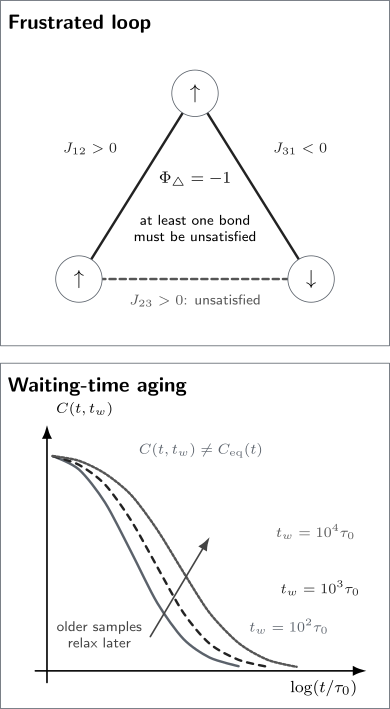
Frustration and aging are distinct. Top: two positive bonds and one negative bond give $\Phi_\triangle=-1$. In the shown ground configuration, the dashed positive bond joins opposite spins and is unsatisfied; the negative bond is satisfied. Bottom: schematic correlations decay more slowly after a longer waiting time. Such a waiting-time dependence diagnoses nonequilibrium aging, but does not by itself establish equilibrium glass order. These are illustrations, not measurements or solutions for a particular material.

Edwards–Anderson model

The short-range benchmark is

$$H_{\mathrm{EA}} = - \sum_{\langle i,j\rangle} J_{ij}S_iS_j - h \sum_iS_i.$$

Typical choices are Gaussian bonds,

$$[J_{ij}]_J = 0, \qquad [J_{ij}^2]_J = J^2,$$

or binary bonds $J_{ij}=\pm J$. The lattice, dimension, boundary conditions, field, and bond distribution are part of the model. Universality can make some critical exponents insensitive to microscopic details, but it does not make finite-size data or transition temperatures convention-free.

For frozen disorder the relevant free energy is

$$F_{\mathrm q}=-k_{\mathrm B}T[\ln Z_J]_J.$$

Here $Z_J$ sums over spins for a fixed sample. Averaging $Z_J$ before taking its logarithm instead describes annealed disorder; Disorder in Quantum Matter derives the difference. In a magnetic alloy, impurity positions are ordinarily fixed on the spin-relaxation timescale.

Rugged landscapes and metastability

For one realization, define the energy of a configuration $\mathbf S$ by $E_J(\mathbf S)$. An extended frustrated system can have many local minima separated by barriers; a single frustrated loop alone does not imply a glass. A minimum relative to single-spin flips need not be stable to collective rearrangements, and the number of minima depends on the chosen move set.

A metastable state is also not automatically a thermodynamic pure state. Metastability is dynamical and time-window dependent; a pure state is an infinite-volume equilibrium concept. Confusing the two turns an optimization landscape into an unsupported phase diagram.

Spin-glass order

Frozen local moments without ordinary magnetization

The uniform magnetization is

$$m = \frac{1}{N} \sum_i [\langle S_i\rangle_J]_J.$$

This averaged quantity vanishes in a zero-field spin glass, but also in a finite spin-flip-symmetric ferromagnet. To distinguish the phases, examine ordinary magnetic order as well as frozen local moments. The Edwards–Anderson order parameter measures the squared local frozen expectation in a selected pure state $\alpha$:

$$q_{\mathrm{EA}} = \frac{1}{N} \sum_i \left[ \langle S_i\rangle_{\alpha,J}^2 \right]_J.$$

The square is taken before the disorder average, so random signs do not cancel. A ferromagnet also has nonzero $q_{\mathrm{EA}}$; glass order requires excluding ordinary uniform or staggered order. At zero field, a finite Gibbs state respects global spin flip and has

$$\langle S_i\rangle_J = 0.$$

For the one-point definition, select an infinite-volume pure state using suitable boundary conditions or a state-selecting source. Take the thermodynamic limit before removing that selection. A uniform magnetic field need not select a particular random spin pattern. Replica correlations provide an alternative that does not require selecting that pattern explicitly.

For equilibrium relaxational dynamics, a corresponding long-time definition is

$$q_{\mathrm{EA}} = \lim_{t\to\infty} \lim_{N\to\infty} C_N(t),$$

where $C_N(t)=N^{-1}\sum_i[\langle S_i(t)S_i(0)\rangle_J]_J$ is the finite-system equilibrium autocorrelation. The state, dynamics and order of limits matter. A finite system with ergodic thermal dynamics eventually forgets its initial spin pattern. A conserved spin component, by contrast, can retain a correlation without any glass transition. In a laboratory that falls out of equilibrium, a finite observation-time plateau indicates freezing, not automatically the infinite-time value.

Two replicas and the overlap

Take two independent equilibrium configurations, $S^{(1)}$ and $S^{(2)}$, subject to the same bond realization. Their spin overlap is

$$q_{12} = \frac{1}{N} \sum_i S_i^{(1)}S_i^{(2)}.$$

For one sample,

$$P_J(q) = \left\langle \delta(q-q_{12}) \right\rangle_J,$$

and the disorder-averaged distribution is

$$P(q) = [P_J(q)]_J.$$

At zero field and finite size, $P_J(q)$ is symmetric under $q\to-q$. A high-temperature paramagnet narrows toward $q=0$. A low-temperature glass develops nonzero overlap weight, but its thermodynamic shape is model dependent.

Equilibrium description	Overlap structure
SK full replica symmetry breaking	A hierarchy with continuous overlap weight and endpoint peaks.
Droplet picture	A symmetry-related pure-state pair gives weight at $\pm q_{\mathrm{EA}}$.
Chaotic-pairs picture	The selected pair can change with sample size; a metastate describes these changes.

The SK description belongs to the infinite-range benchmark. The alternatives concern the organization of short-range equilibrium states, not arbitrary fits to one finite histogram. At finite size, every picture can produce rounded peaks and central weight. Even independent paramagnetic spins have $\langle q_{12}^2\rangle=1/N$, so nonzero overlap in one small sample is not sufficient.

The overlap is not a conventional local observable in one replica, but it is operational in simulations and in coupled-copy protocols.

Spin-glass susceptibility and correlation length

At zero field, the spin-glass susceptibility is

$$\chi_{\mathrm{SG}} = \frac{1}{N} \sum_{i,j} \left[ \langle S_iS_j\rangle_J^2 \right]_J.$$

For two independent replicas with common disorder,

$$\chi_{\mathrm{SG}} = N \left[ \langle q_{12}^2\rangle_J \right]_J.$$

In a field, remove the local magnetizations $m_i=\langle S_i\rangle_J$ before forming the squared correlation. Define

$$G_{ij}^{\mathrm c} =\langle S_iS_j\rangle_J -m_i m_j.$$

The connected spin-glass susceptibility is

$$\chi_{\mathrm{SG}}^{\mathrm c} =\frac1N\sum_{i,j}[(G_{ij}^{\mathrm c})^2]_J.$$

Define the spatial glass correlator

$$G_{\mathrm{SG}}(\mathbf r) = \frac{1}{N} \sum_i \left[ \langle S_iS_{i+\mathbf r} \rangle_J^2 \right]_J$$

at zero field, and let $\widetilde G_{\mathrm{SG}}(\mathbf k)$ be its Fourier transform. For a periodic cubic sample of $L$ sites per side, set the lattice spacing to one and choose $\mathbf k_{\min}=(2\pi/L,0,\ldots)$, with magnitude $k_{\min}$. A common second-moment finite-size length is

$$\xi_L = \frac{1}{ 2\sin(k_{\min}/2) } \left[ \frac{ \widetilde G_{\mathrm{SG}}(\mathbf 0) }{ \widetilde G_{\mathrm{SG}}(\mathbf k_{\min}) } - 1 \right]^{1/2}.$$

Crossings of $\xi_L/L$ across several sizes are far stronger evidence for a thermodynamic transition than a single broad peak in susceptibility. The crossing must survive longer equilibration, larger sizes and corrections to scaling (Ballesteros et al., 2000).

Observing freezing

A frequency-dependent susceptibility cusp, field-cooled/zero-field-cooled splitting, remanence and aging all indicate slow magnetic dynamics. Nonlinear susceptibility scaling and local probes of frozen random moments add complementary information. Independent blocked nanoparticles or moving domain walls can reproduce several of these signatures; cooperative freezing requires comparing temperature, field and time dependence with those mechanisms.

The characteristic time is often fitted either to critical slowing,

$$\tau = \tau_0 \left| \frac{ T_f-T_g }{ T_g } \right|^{-z\nu},$$

or to a Vogel–Fulcher form,

$$\tau = \tau_0 \exp\!\left[ \frac{A}{ T_f-T_0 } \right].$$

Over a narrow frequency interval, both can fit. The attempt time $\tau_0$ and fitted temperatures must be physically plausible and stable when the fit interval changes; a good fit alone does not select the mechanism. In the Vogel–Fulcher expression, $A$ is measured in temperature units.

Sherrington–Kirkpatrick mean-field benchmark

The infinite-range Ising model is

$$H_{\mathrm{SK}} = - \sum_{i<j} J_{ij}S_iS_j - h \sum_iS_i,$$

with independent Gaussian bonds whose mean and variance are

$$\begin{aligned} [J_{ij}]_J&=J_0/N,\\ \operatorname{Var}_J(J_{ij})&=J^2/N. \end{aligned}$$

The $N^{-1/2}$ width gives an extensive thermodynamic free energy. A fixed unoptimized spin configuration has random energy fluctuations of order $\sqrt N$, while equilibrium selection among exponentially many configurations produces an energy of order $N$.

Set $J_0=0$ and write $\beta=(k_{\mathrm B}T)^{-1}$. Define the dimensionless effective field

$$u(z)=\beta(J\sqrt q\,z+h).$$

In the replica-symmetric approximation, the overlap satisfies

$$q=\int Dz\,\tanh^2u(z),$$

where $Dz=e^{-z^2/2}dz/\sqrt{2\pi}$ and the integral covers the real line. At $h=0$, this reduces to the zero-field equation.

At $h=0$, linearizing at small $q$ gives

$$q \simeq (\beta J)^2q,$$

and therefore

$$k_{\mathrm B}T_c = J.$$

For the same self-consistent $q$, the replica-symmetric free-energy density is

$$f_{\mathrm{RS}} =-\frac{\beta J^2}{4}(1-q)^2 -\frac1\beta\int Dz\,\ln[2\cosh u(z)].$$

Its local stability against overlap fluctuations is controlled by the replicon eigenvalue

$$\lambda_{\mathrm R} =1-(\beta J)^2\int Dz\,\operatorname{sech}^4u(z).$$

The de Almeida–Thouless boundary satisfies

$$\lambda_{\mathrm R} = 0.$$

A negative replicon signals instability of this saddle. The de Almeida–Thouless criterion is the standard SK mean-field stability result; it does not establish a transition in a short-range magnet. The zero-field SK glass requires the Parisi hierarchy below $T_c$.

Replica method and equilibrium states

The quenched logarithm

The obstacle is the disorder average of $\ln Z_J$. For positive integer $n$,

$$Z_J^n = \prod_{a=1}^{n} \sum_{\{S_i^a\}} e^{-\beta H_J[S^a]},$$

which introduces $n$ copies sharing the same disorder. The formal identity is

$$[\ln Z_J]_J = \lim_{n\to0} \frac{ [Z_J^n]_J-1 }{ n }.$$

The procedure is:

1. compute $[Z_J^n]_J$ for positive integer $n$;
2. express the answer in terms of replica overlaps;
3. analytically continue away from integer $n$;
4. take $n\to0$.

Step 3 is the delicate one. Values at positive integers do not by themselves determine a unique analytic continuation. The replica trick, or replica method, is a powerful formal calculus whose predictions must be checked against controlled solutions, rigorous methods, or independent numerics.

Overlap matrix

Disorder averaging couples replicas through

$$q_{ab} = \frac{1}{N} \sum_i S_i^aS_i^b, \qquad a\neq b.$$

A replica-symmetric ansatz sets

$$q_{ab} = q$$

for every $a\neq b$. The low-temperature SK saddle violates this permutation symmetry in a hierarchical way. In the full Parisi construction, the discrete hierarchy becomes a function

$$q(x), \qquad 0\leq x\leq1,$$

related to the distribution of overlaps among equilibrium states. Replica symmetry breaking is therefore more than “many local minima”: it is a specific organization of equilibrium Gibbs weight.

What is established and what is not

The Parisi variational formula gives the exact thermodynamic free energy of the SK model (Talagrand, 2006). Guerra established the matching variational bound needed for the program, and Talagrand proved the formula. These results vindicate a central mean-field prediction without turning every formal $n\to0$ manipulation into a general theorem.

For the three-dimensional short-range Edwards–Anderson model:

• numerical work strongly supports a finite-temperature zero-field transition for Ising spins;
• the number and organization of low-temperature pure states remain debated;
• droplet, replica-symmetry-breaking, chaotic-pairs, and related metastate descriptions make different thermodynamic predictions;
• the existence of a de Almeida–Thouless-like line in a field is not settled.

The distinction between mean-field and short-range systems is essential: a solved infinite-range free energy does not determine the state structure of a laboratory magnet.

Aging and slow dynamics

Waiting-time protocol

Quench the system from high temperature to a low measuring temperature, wait for time $t_w$, and then observe for an additional lag $t$. Define

$$C(t,t_w) = \frac{1}{N} \sum_i \left[ \left\langle S_i(t_w+t) S_i(t_w) \right\rangle \right]_J.$$

In equilibrium, time-translation invariance gives

$$C(t,t_w) = C_{\mathrm{eq}}(t).$$

In an aging system,

$$\frac{\partial C(t,t_w)}{ \partial t_w } \neq 0.$$

Older samples commonly decorrelate more slowly. A useful decomposition is

$$\begin{aligned} C(t,t_w)&\simeq C_{\mathrm{st}}(t)+C_{\mathrm{ag}}(u),\\ u&=h(t_w+t)/h(t_w), \end{aligned}$$

where $h$ is a model- and protocol-dependent clock. Simple $t/t_w$ aging is not universal; subaging and multiple sectors are possible. The controlled spherical $p$-spin solution of Cugliandolo and Kurchan (1993) is one model where aging and nontrivial response ratios can be derived.

Response and fluctuation–dissipation ratio

For response functions, use absolute times $t_f>s$ and the perturbation $\delta H(s)=-\sum_i h_i(s)S_i$. Distinguish the absolute-time correlator from the lag–waiting-time notation above:

$$C_{\mathrm{abs}}(t_f,s) = C(t_f-s,s).$$

Define

$$R(t_f,s) = \frac{1}{N} \sum_i \left. \frac{ \delta \langle S_i(t_f)\rangle }{ \delta h_i(s) } \right|_{h=0}$$

with the same spin and disorder averaging as the correlator. The formulas here use classical relaxational dynamics, zero applied field and the spin-flip-symmetric ensemble. If a nonzero mean is present, use connected correlations. At equilibrium, the classical fluctuation–dissipation theorem gives

$$k_{\mathrm B}T R(t_f,s) = \frac{ \partial C_{\mathrm{abs}}(t_f,s) }{ \partial s }.$$

The derivative holds the final absolute time $t_f$ fixed. In the lag–waiting-time coordinates, it therefore differentiates both arguments: $\partial_s C_{\mathrm{abs}}=(\partial_{t_w}-\partial_t)C(t,t_w)$ evaluated at $t=t_f-s$ and $t_w=s$. A derivative at fixed lag would vanish in equilibrium and would not give the response.

Out of equilibrium, define

$$k_{\mathrm B}T R(t_f,s) = X(t_f,s) \frac{ \partial C_{\mathrm{abs}}(t_f,s) }{ \partial s }.$$

Fast quasi-equilibrated modes often have $X\simeq1$, while slow aging sectors can have $X\neq1$. An effective temperature

$$T_{\mathrm{eff}} = \frac{T}{X}$$

is meaningful only if the long-time ratio is stable, observable independent within a sector, and consistent with a weak thermometer. A curved response–correlation plot or frequency-dependent $X$ is not one scalar temperature.

Fluctuation–Dissipation Relation explains the equilibrium theorem, quantum ordering conventions, and bath assumptions. Here its violation is used as a nonequilibrium glass diagnostic.

Memory and rejuvenation

In a temperature-stop protocol:

1. cool to $T_1<T_g$ and wait;
2. cool further to $T_2$;
3. reheat through $T_1$.

The response can resume aging at $T_2$ as though newly prepared, called rejuvenation, while recovering a dip or relaxation imprint near $T_1$, called memory. These effects suggest a hierarchy of times or length scales. They do not uniquely select a Parisi state hierarchy over real-space droplet growth.

For a real-space activated description, let $L$ be a coherence length in microscopic length units. Its age dependence is

$$L(t,T) \sim \left[ \frac{ k_{\mathrm B}T }{ \Delta } \ln\!\left( \frac{t}{\tau_0} \right) \right]^{1/\psi}$$

for activated barriers

$$B(L) \sim \Delta L^\psi.$$

This logarithmic form is asymptotic and model dependent. Experimental length scales can remain far below those needed to distinguish competing thermodynamic pictures.

Equilibrium, structural glasses and quantum models

Equilibrium, kinetics, and the order of limits

An equilibrium Gibbs measure is mathematically defined even when an experiment cannot sample it. Comparing its predictions to a glass requires checking the observation timescale. A glass exposes the order-of-limits problem:

$$\lim_{t_{\mathrm{obs}}\to\infty} \lim_{N\to\infty} \quad\text{versus}\quad \lim_{N\to\infty} \lim_{t_{\mathrm{obs}}\to\infty}.$$

For any finite system with ergodic dynamics and finite barriers, sufficiently long observation restores equilibrium. If barriers grow with size, the thermodynamic limit can produce broken ergodicity before the infinite-time limit is taken.

Thermodynamic statements use the equilibrium measure and controlled limits. Aging statements use a preparation protocol and two-time observables. Neither should be substituted for the other.

Structural glasses

A structural glass is formed when a liquid avoids crystallization and falls out of equilibrium as its structural relaxation time exceeds the experimental window. It normally has no externally quenched $J_{ij}$. Disorder is self-generated by particle positions.

A common single-particle correlator uses the displacement $\Delta\mathbf r_j(t)=\mathbf r_j(t)-\mathbf r_j(0)$:

$$F_s(\mathbf k,t) = \frac{1}{N} \sum_j \left\langle e^{ i\mathbf k\cdot\Delta\mathbf r_j(t) } \right\rangle.$$

Supercooled liquids often show a two-step decay, a plateau from transient caging, growing dynamic heterogeneity, and aging below the operational glass temperature. Mean-field $p$-spin models and replica ideas illuminate these features; whether and how an ideal equilibrium glass transition occurs depends on the model and is a separate question from kinetic arrest. The laboratory $T_g$ is rate dependent; it is not automatically an equilibrium critical temperature.

Quantum spin glasses

The transverse-field Edwards–Anderson model is

$$H_{\mathrm{QEA}}=-\sum_{\langle i,j\rangle}J_{ij}\sigma_i^z\sigma_j^z -\Gamma\sum_i\sigma_i^x.$$

The transverse field produces tunneling between classical configurations and can drive a zero-temperature transition. Under an imaginary-time mapping, the quenched spatial bond is repeated along the entire imaginary-time direction. The effective classical disorder is therefore perfectly correlated in imaginary time, not an ordinary uncorrelated $(d+1)$-dimensional random magnet.

Quantum fluctuations do not guarantee rapid equilibration or optimization. Small avoided gaps, localization in configuration space, dissipation, longitudinal random fields, and finite annealing schedules can dominate. Transverse-Field Ising Model develops the clean model and its quantum critical point; the random frustrated extension adds an active research layer.

Equilibration is particularly demanding in glass simulations. Independent starts, replica exchange, overlap moments and the distribution of relaxation times across disorder samples help expose false convergence. Extend runs and compare sizes before interpreting a crossing as thermodynamic order; Finite-Size Scaling in Numerics describes that analysis.

Exercises

1. Frustration on a triangle

For three Ising spins with

$$J_{12}=J_{23}=J,\qquad J_{31}=-J,$$

with $J>0$, show that every configuration leaves at least one bond unsatisfied and find the ground-state energy.

Solution

The loop product is

$$\Phi_\triangle = \operatorname{sgn} (J_{12}J_{23}J_{31}) = -1.$$

If all bonds were satisfied, the required pair products would be

$$\begin{aligned} S_1S_2&=S_2S_3=+1,\\ S_3S_1&=-1. \end{aligned}$$

Multiplying the left sides gives $+1$, while multiplying the right sides gives $-1$, a contradiction.

Each satisfied bond contributes $-J$ and one unsatisfied bond contributes $+J$, so

$$E_{\min} = -J-J+J = -J.$$

There are six ground configurations: choose which bond is unsatisfied and apply the global spin flip.

2. Replica overlap and susceptibility

At zero field, prove

$$\chi_{\mathrm{SG}} = N \left[ \langle q_{12}^2\rangle_J \right]_J.$$

Solution

Write $A_{ij}^{(a)}=S_i^{(a)}S_j^{(a)}$ and expand the squared overlap:

$$\langle q_{12}^2\rangle_J = \frac{1}{N^2} \sum_{i,j} \left\langle A_{ij}^{(1)}A_{ij}^{(2)} \right\rangle_J.$$

The replicas are thermally independent conditional on the same bonds, so

$$\left\langle A_{ij}^{(1)}A_{ij}^{(2)} \right\rangle_J = \langle S_iS_j\rangle_J^2.$$

Multiplying by $N$ and averaging over disorder yields the stated susceptibility.

3. SK transition temperature

Linearize

$$q = \int Dz\, \tanh^2( \beta J\sqrt q\,z )$$

near $q=0$ and determine $T_c$.

Solution

For small argument,

$$\tanh x = x+O(x^3).$$

Hence

$$\begin{aligned} q &= \int Dz\, \left[ \beta^2J^2qz^2 + O(q^2) \right] \\ &= \beta^2J^2q + O(q^2), \end{aligned}$$

because $\int Dz\,z^2=1$. A nonzero infinitesimal solution appears when

$$\beta_cJ = 1,$$

so

$$k_{\mathrm B}T_c = J.$$

This is the zero-field, zero-mean-coupling SK result, not a universal laboratory freezing temperature.

4. Read a fluctuation–dissipation plot

For the Ising autocorrelation, $C_{\mathrm{abs}}(t_f,t_f)=1$. At a fixed final absolute time $t_f$, vary the waiting time $t_w<t_f$ and plot $k_{\mathrm B}T\chi_{\mathrm{abs}}$ against $C=C_{\mathrm{abs}}(t_f,t_w)$, where

$$\chi_{\mathrm{abs}}(t_f,t_w) = \int_{t_w}^{t_f} ds\,R(t_f,s).$$

Suppose the fast sector has slope $-1$ and the slow sector has slope $-0.40$. Find the slow-sector $X$ and $T_{\mathrm{eff}}$.

Solution

Equilibrium integration gives

$$k_{\mathrm B}T\chi_{\mathrm{abs}} = 1-C,$$

so its slope is $-1$. At fixed $t_f$, differentiation with respect to $t_w$ gives $\partial_{t_w}\chi_{\mathrm{abs}}=-R(t_f,t_w)$. Combining this with the defining FDT ratio gives, in a sector with constant $X$,

$$\frac{ d(k_{\mathrm B}T\chi_{\mathrm{abs}}) }{ dC } = -X.$$

Therefore

$$X = 0.40,$$

and

$$T_{\mathrm{eff}} = \frac{T}{X} = 2.5T.$$

This interpretation still requires the same asymptotic slope for several observables and a consistent thermometer response. A plot made instead at fixed $t_w$ while varying $t_f$ needs an additional common or asymptotic relation $X=X(C)$ before its slope can be read this way. If a different observable’s correlator is normalized by a nonunit equal-time variance, its susceptibility must be divided by that same variance.

5. Order of limits

Explain why a finite zero-field Ising spin glass can have

$$\langle S_i\rangle_J=0$$

even below a transition. Does nonzero $[\langle q_{12}^2\rangle_J]_J$ alone establish order? Evaluate it for $N$ independent unbiased Ising spins.

Solution

The finite Hamiltonian is invariant under the global transformation

$$S_i \longmapsto -S_i.$$

The Gibbs measure therefore pairs every configuration with its flipped partner, forcing each odd one-point function to vanish.

The overlap changes sign if only one replica is flipped, but its square is invariant:

$$q_{12}^2 \longmapsto q_{12}^2.$$

For independent unbiased spins, only equal-site terms survive in the squared-overlap sum, giving $\langle q_{12}^2\rangle=N/N^2=1/N$. Thus it is nonzero even in a finite paramagnet, but vanishes as $N\to\infty$. Glass correlations must be identified by their scaling. A pure-state one-point definition instead takes the thermodynamic limit before removing a suitable selecting source or boundary condition.

References

• H. G. Ballesteros, A. Cruz, L. A. Fernández, et al., “Critical Behavior of the Three-Dimensional Ising Spin Glass,” Physical Review B 62, 14237–14245 (2000), doi:10.1103/PhysRevB.62.14237. Provides finite-size correlation-length evidence for a nonzero-temperature transition.
• L. Berthier and G. Biroli, “Theoretical Perspective on the Glass Transition and Amorphous Materials,” Reviews of Modern Physics 83, 587–645 (2011), doi:10.1103/RevModPhys.83.587. Reviews structural-glass dynamics, heterogeneity, aging, and competing theories.
• K. Binder and A. P. Young, “Spin Glasses: Experimental Facts, Theoretical Concepts, and Open Questions,” Reviews of Modern Physics 58, 801–976 (1986), doi:10.1103/RevModPhys.58.801. Reviews models, experiments, dynamics, simulations, and conceptual pitfalls.
• L. F. Cugliandolo and J. Kurchan, “Analytical Solution of the Off-Equilibrium Dynamics of a Long-Range Spin-Glass Model,” Physical Review Letters 71, 173–176 (1993), doi:10.1103/PhysRevLett.71.173. Derives aging and response–correlation structure in a controlled mean-field model.
• J. R. L. de Almeida and D. J. Thouless, “Stability of the Sherrington–Kirkpatrick Solution of a Spin Glass Model,” Journal of Physics A: Mathematical and General 11, 983–990 (1978), doi:10.1088/0305-4470/11/5/028. Derives the replica-symmetric stability boundary.
• S. F. Edwards and P. W. Anderson, “Theory of Spin Glasses,” Journal of Physics F: Metal Physics 5, 965–974 (1975), doi:10.1088/0305-4608/5/5/017. Introduces the short-range random-bond model and frozen-local-moment order parameter.
• D. S. Fisher and D. A. Huse, “Ordered Phase of Short-Range Ising Spin-Glasses,” Physical Review Letters 56, 1601–1604 (1986), doi:10.1103/PhysRevLett.56.1601. Develops the droplet scaling alternative to mean-field state structure.
• J. A. Mydosh, “Spin Glasses: Redux: An Updated Experimental/Materials Survey,” Reports on Progress in Physics 78, 052501 (2015), doi:10.1088/0034-4885/78/5/052501. Reviews material classes, experimental signatures, and persistent ambiguities.
• C. M. Newman and D. L. Stein, “Ordering and Broken Symmetry in Short-Ranged Spin Glasses,” Journal of Physics: Condensed Matter 15, R1319–R1364 (2003), doi:10.1088/0953-8984/15/32/202. Develops metastates and critiques direct mean-field extrapolation to finite dimensions.
• G. Parisi, “Infinite Number of Order Parameters for Spin-Glasses,” Physical Review Letters 43, 1754–1756 (1979), doi:10.1103/PhysRevLett.43.1754. Introduces the continuous replica-symmetry-breaking hierarchy.
• G. Parisi, “Order Parameter for Spin-Glasses,” Physical Review Letters 50, 1946–1948 (1983), doi:10.1103/PhysRevLett.50.1946. Connects the Parisi function to physical overlap probabilities.
• D. Sherrington and S. Kirkpatrick, “Solvable Model of a Spin-Glass,” Physical Review Letters 35, 1792–1796 (1975), doi:10.1103/PhysRevLett.35.1792. Defines the infinite-range mean-field benchmark.
• M. Talagrand, “The Parisi Formula,” Annals of Mathematics 163, 221–263 (2006), doi:10.4007/annals.2006.163.221. Proves the Parisi free-energy formula for the SK model.

Further Reading

• M. Mézard, G. Parisi, and M. A. Virasoro, Spin Glass Theory and Beyond, World Scientific, 1987, doi:10.1142/0271. A detailed development of replicas, mean-field theory, and overlap structure.
• J. A. Mydosh, Spin Glasses: An Experimental Introduction, Taylor & Francis, 1993, doi:10.1201/9780429499517. A materials- and protocol-centered experimental account.
• A. P. Young, ed., Spin Glasses and Random Fields, World Scientific, 1998, doi:10.1142/3517. Reviews droplet, replica, dynamics, and random-field perspectives.