Fluctuation–Dissipation Relation

The fluctuation–dissipation relation says that, in thermal equilibrium, noise and damping are not independent. The same microscopic degrees of freedom that exert random forces also absorb energy from a driven system.

In open quantum systems this relation is used to check thermal master equations, connect bath spectra to dissipative response, interpret vacuum noise, and avoid treating equilibrium noise as an arbitrary fitting function. The source-to-observable susceptibility is introduced in Green Functions and Response Preview and developed for many-body systems in the Kubo Formula. The Caldeira–Leggett Model is the standard oscillator-bath example where the same spectral density produces both a damping kernel and a thermal force-noise kernel.

The scope here is practical: how the relation appears in bath spectra, damping kernels, transition rates, and weak-coupling open-system modeling. Fluctuation–Dissipation Theorem gives the general many-body proof and explains the matrix, momentum, and static-response versions. The equilibrium static identities and the distinction between ordinary variance and Kubo–Mori covariance are developed in Fluctuations and Susceptibilities.

Equilibrium Noise and Energy Absorption

At equilibrium:

fluctuations reveal what the bath can do spontaneously;
dissipation reveals how the bath absorbs energy when driven.

The fluctuation–dissipation relation connects these two descriptions. It is not a generic statement about every noisy environment. It relies on equilibrium, stationarity, and linear response.

If a reservoir is driven, inverted, feedback-controlled, measurement-conditioned, or made of multiple baths at different temperatures, the equilibrium relation generally fails.

Noise and Response Definitions

Let $B(t)$ be a centered Hermitian bath observable in a thermal stationary state, with its mean subtracted. The formulas below describe the dynamical spectrum at nonzero frequency; a zero-frequency elastic contribution needs separate treatment. The symmetrized spectrum is

$$S_{BB}^{\mathrm{sym}}(\omega) = \frac12 \int_{-\infty}^{\infty} dt\, e^{i\omega t} \langle \{B(t),B(0)\}\rangle.$$

Now perturb the bath by a weak classical source coupled to $B$:

$$H_{\mathrm{drive}}(t) = -f(t)B.$$

The retarded susceptibility is defined by

$$\chi_{BB}^R(t) = \frac{i}{\hbar} \theta(t) \langle [B(t),B(0)]\rangle.$$

It gives the linear response

$$\delta\langle B(t)\rangle = \int_{-\infty}^{\infty} dt'\, \chi_{BB}^R(t-t')f(t').$$

Use $\chi^R(\omega)=\int dt\,e^{i\omega t}\chi^R(t)$, the same transform as for noise. With the specified source $-fB$, a passive equilibrium bath has $\operatorname{Im}\chi^R(\omega)\ge0$ for $\omega>0$. The equilibrium relation is

$$S_{BB}^{\mathrm{sym}}(\omega) = \hbar \coth\!\left( \frac{\beta\hbar\omega}{2} \right) \operatorname{Im}\chi_{BB}^R(\omega).$$

Some books define the retarded susceptibility with an extra minus sign. Then the displayed formula changes sign accordingly. The physical spectrum must remain nonnegative.

Relation to Ordered Spectra

The ordered spectrum is

$$S_{BB}(\omega) = \int_{-\infty}^{\infty} dt\, e^{i\omega t} \langle B(t)B(0)\rangle.$$

For a Hermitian operator,

$$S_{BB}^{\mathrm{sym}}(\omega) = \frac12 \left[ S_{BB}(+\omega) + S_{BB}(-\omega) \right].$$

Thermal equilibrium also gives the Kubo–Martin–Schwinger relation

$$S_{BB}(-\omega) = e^{-\beta\hbar\omega} S_{BB}(+\omega), \qquad \omega>0.$$

The dissipative response is tied to the antisymmetric part:

$$S_{BB}(+\omega)-S_{BB}(-\omega) = 2\hbar\, \operatorname{Im}\chi_{BB}^R(\omega)$$

with the susceptibility convention used on this page. Combining this identity with the KMS relation gives

$$\frac{ S_{BB}(+\omega)+S_{BB}(-\omega) }{ S_{BB}(+\omega)-S_{BB}(-\omega) } = \coth\!\left( \frac{\beta\hbar\omega}{2} \right),$$

which is the fluctuation–dissipation relation in spectral form.

Classical High-Temperature Limit

When

$$\beta\hbar|\omega|\ll1,$$

the thermal factor becomes

$$\hbar \coth\!\left( \frac{\beta\hbar\omega}{2} \right) \approx \frac{2k_BT}{\omega}.$$

The relation becomes the classical fluctuation–dissipation form

$$S_{BB}^{\mathrm{sym}}(\omega) \approx \frac{2k_BT}{\omega} \operatorname{Im}\chi_{BB}^R(\omega).$$

This is why thermal noise is proportional to temperature in classical regimes. The factor multiplying $T$ depends on what variable is being measured and on the response function convention.

Quantum Low-Temperature Limit

When

$$\beta\hbar|\omega|\gg1,$$

the factor approaches

$$\coth\!\left( \frac{\beta\hbar\omega}{2} \right) \longrightarrow \operatorname{sgn}(\omega).$$

The symmetrized spectrum does not vanish at zero temperature:

$$S_{BB}^{\mathrm{sym}}(\omega) \longrightarrow \hbar |\operatorname{Im}\chi_{BB}^R(\omega)|.$$

This is the spectral language of zero-point fluctuations. However, zero-temperature symmetrized noise should not be confused with the ability of the bath to excite a system. The ordered negative-frequency spectrum is suppressed for an ordinary ground-state bath.

Detailed Balance and Master Equations

For a two-level system of transition frequency $\omega_0>0$, weakly coupled to a thermal bath,

$$\Gamma_\downarrow \propto S_{BB}(+\omega_0), \qquad \Gamma_\uparrow \propto S_{BB}(-\omega_0).$$

The KMS relation gives

$$\frac{\Gamma_\uparrow}{\Gamma_\downarrow} = e^{-\beta\hbar\omega_0}.$$

This is the rate-level form of Detailed Balance. It makes the Gibbs state stationary for a properly derived single-bath weak-coupling generator. Relaxation to a unique Gibbs state additionally requires that the transitions connect all relevant sectors; dark states or conserved quantities can prevent uniqueness.

The fluctuation–dissipation relation adds a response interpretation: the same bath spectral asymmetry that fixes upward and downward rates also fixes the relation between equilibrium noise and dissipative susceptibility.

Example: Johnson–Nyquist Noise

For a resistor with resistance $R$, the two-sided angular-frequency symmetrized voltage noise is often written

$$S_{VV}^{\mathrm{sym}}(\omega) = \hbar\omega R \coth\!\left( \frac{\beta\hbar\omega}{2} \right),$$

with this convention. In the classical high-temperature limit,

$$S_{VV}^{\mathrm{sym}}(\omega) \approx 2Rk_BT.$$

In one-sided ordinary-frequency notation this same result is commonly written with the familiar factor $4Rk_BT$. The physics is the same; the spectral convention is different.

At low temperature, the symmetrized voltage noise retains a quantum contribution proportional to $\hbar R|\omega|$. Whether that noise can excite a detector depends on the ordered spectrum and the detector’s coupling.

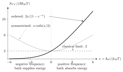
Thermal voltage noise of an ideal frequency-independent resistor. The ordered spectrum is $S_{VV}(\omega)=2R\hbar\omega/(1-e^{-\beta\hbar\omega})$; the gray curve averages its positive- and negative-frequency values. Only the central region $|\hbar\omega|\ll k_BT$ resembles classical white noise. The negative-frequency tail falls because the bath has less energy available to excite a detector.

Example: Damped Oscillator

For a harmonic coordinate with mass $m$, frequency $\Omega$, and Ohmic friction rate $\gamma$,

$$\chi_{xx}^R(\omega)=\frac1{m(\Omega^2-\omega^2-i\gamma\omega)}.$$

The imaginary part is positive for $\omega>0$, giving a useful sign check. A weak force $f$ produces

$$\delta\langle x(\omega)\rangle = \chi_{xx}^R(\omega)f(\omega).$$

The fluctuation–dissipation relation gives

$$S_{xx}^{\mathrm{sym}}(\omega) = \hbar \coth\!\left( \frac{\beta\hbar\omega}{2} \right) \operatorname{Im}\chi_{xx}^R(\omega),$$

with the stated source and Fourier conventions. Equivalently, the symmetrized force noise is $S_{FF}^{\mathrm{sym}}=m\gamma\hbar\omega\coth(\beta\hbar\omega/2)$ and $S_{xx}=|\chi_{xx}^R|^2 S_{FF}$. At high temperature this becomes $S_{FF}=2m\gamma k_BT$, recovering classical thermal Langevin noise.

This is the oscillator version of the same principle used in bath modeling: equilibrium fluctuations are weighted by the bath’s ability to absorb energy.

What the Relation Does Not Say

The fluctuation–dissipation relation does not mean every noise model must include a matching damping term. It means that an equilibrium thermal bath with linear response has constrained noise and dissipation.

It does not apply without additional work to:

• nonthermal driven reservoirs;
• active or inverted media;
• feedback-controlled baths;
• measurement-conditioned trajectories;
• classical technical noise from electronics or drift;
• multiple reservoirs at different temperatures;
• aging, glassy, or nonstationary environments;
• an approximate bare-system spectrum paired with an unrelated response function at strong coupling.

The exact equilibrium relation itself remains valid at strong coupling when the correlations and response are calculated for the same full equilibrium Hamiltonian. What fails is an inconsistent separation into bare system and bath quantities. Out of equilibrium, no general equilibrium FDR follows.

At $\omega=0$, conserved or nondecaying fluctuations can produce a delta function while the corresponding dissipative response vanishes. One cannot recover that elastic weight by simply dividing a vanishing commutator spectrum by $1-e^{-\beta\hbar\omega}$. See the static-response caveat for this limit.

Exercises

KMS to Detailed Balance

Use

$$S(-\omega) = e^{-\beta\hbar\omega}S(+\omega)$$

to derive the upward-to-downward rate ratio for a two-level system.

Solution

With the convention on this page,

$$\Gamma_\downarrow\propto S(+\omega_0), \qquad \Gamma_\uparrow\propto S(-\omega_0).$$

Therefore

$$\frac{\Gamma_\uparrow}{\Gamma_\downarrow} = \frac{S(-\omega_0)}{S(+\omega_0)} = e^{-\beta\hbar\omega_0}.$$

Algebraic FDR Factor

Let $x=\beta\hbar\omega$ and assume $S(-\omega)=e^{-x}S(+\omega)$. Show that

$$\frac{S(+\omega)+S(-\omega)} {S(+\omega)-S(-\omega)} = \coth\!\left(\frac{x}{2}\right).$$

Solution

Substitute $S(-\omega)=e^{-x}S(+\omega)$:

$$\frac{S(+\omega)+S(-\omega)} {S(+\omega)-S(-\omega)} = \frac{1+e^{-x}}{1-e^{-x}}.$$

Multiplying numerator and denominator by $e^{x/2}$ gives

$$\frac{e^{x/2}+e^{-x/2}} {e^{x/2}-e^{-x/2}} = \coth\!\left(\frac{x}{2}\right).$$

High-Temperature Johnson Noise

Starting from

$$S_{VV}^{\mathrm{sym}}(\omega) = \hbar\omega R \coth\!\left( \frac{\beta\hbar\omega}{2} \right),$$

show the high-temperature two-sided angular-frequency limit.

Solution

For $\beta\hbar|\omega|\ll1$,

$$\coth\!\left( \frac{\beta\hbar\omega}{2} \right) \approx \frac{2}{\beta\hbar\omega}.$$

Thus

$$S_{VV}^{\mathrm{sym}}(\omega) \approx \hbar\omega R \frac{2}{\beta\hbar\omega} = 2Rk_BT.$$

Symmetrized Versus Ordered Noise

At zero temperature an equilibrium bath has no negative-frequency ordered noise for $\omega>0$ in this convention, but the symmetrized spectrum is nonzero. Explain why these statements are compatible.

Solution

The ordered negative-frequency spectrum describes the bath supplying energy to a system. At zero temperature an ordinary equilibrium bath cannot supply energy at positive transition frequency, so that part is suppressed.

The symmetrized spectrum is the average of ordered positive- and negative-frequency spectra:

$$S^{\mathrm{sym}}(\omega) = \frac12 \left[ S(+\omega)+S(-\omega) \right].$$

At zero temperature $S(-\omega)$ may vanish for $\omega>0$, but $S(+\omega)$ need not. The bath can still absorb energy, and the symmetrized spectrum records zero-point fluctuations associated with that response.

References

• H.-P. Breuer and F. Petruccione, The Theory of Open Quantum Systems, Oxford University Press (2002).
• H. B. Callen and T. A. Welton, “Irreversibility and generalized noise,” Physical Review 83, 34–40 (1951).
• A. A. Clerk, M. H. Devoret, S. M. Girvin, F. Marquardt, and R. J. Schoelkopf, “Introduction to quantum noise, measurement, and amplification,” Reviews of Modern Physics 82, 1155–1208 (2010), doi:10.1103/RevModPhys.82.1155.
• C. W. Gardiner and P. Zoller, Quantum Noise, Springer (2004).
• R. Kubo, “Statistical-mechanical theory of irreversible processes. I,” Journal of the Physical Society of Japan 12, 570–586 (1957).
• R. Kubo, “The fluctuation-dissipation theorem,” Reports on Progress in Physics 29, 255–284 (1966).
• U. Weiss, Quantum Dissipative Systems, World Scientific (2012).